Introduction
This is a guide on how to use the program PyMCA for X-ray fluorescence (XRF) imaging analysis at the NanoMAX beamline. PyMCA is developed at ESRF by V. Armando Solé. It can be downloaded from SourceForge, as a standalone program for Windows or MAC. You can also install is as a python package if you are developing in python. Download and installation instructions are found at https://sourceforge.net/projects/pymca/
If you are using Anaconda as a python environment for data analysis, you can install PyMCA as python package with the command conda install -c conda-forge pymca silx. The conda installation is hosted at https://anaconda.org/conda-forge/pymca
Experimental data from NanoMAX is stored in a raw directory. However, the raw data is not readily readable by PyMCA. Therefore, you will find data in a /process/XRF_pymca directory, converted to suit PyMCA analysis. Raw and converted data is stored on the MAX IV file storage in the following way: /data/visitors/nanomax/[proposal]/[session]/ with sub directories raw, process, photos, macros and logs. The electronic logbook is typically stored in the logs directory
The guide will help you to load experimental data into PyMCA, to do a first spectral fitting of elements in your sample and to generate images of elements. The images will show element distribution either qualitatively or if sample conditions allow also quantitatively. The typical data analysis procedure consists of these steps.
- Open XRF image data in PyMCA.
- View the XRF sum spectrum.
- Load a fitting configuration template file.
- Adjust parameters in the fitting configuration.
- Run a fit and iteratively adjust parameters to reach a good spectral fit.
- Save the optimized configuration to a new configuration file.
- Run a Fast XRF stack fitting to produce elemental images with relative concentrations.
- Optionally use an XRF reference sample to update the configuration file to allow for element concentration quantification.
- Re-run step 7 with the referenced configuration file to produce images with concentrations expressed as nanograms/mm2.
- Optionally generate three-colour maps of elements.
All steps are illustrated in the following pages as a step-by-step guide with PyMCA screen shots.
Note that this guide is not describing what is a good or less good fit. It is only intending to help you to get started with the practical moments of XRF imaging analysis.
Useful links:
- PyMCA home page: http://pymca.sourceforge.net/
- PyMCA documentation: http://www.silx.org/doc/PyMca/latest/index.html
- PyMCA mailing list: https://sourceforge.net/p/pymca/mailman/
- PyMCA program download: https://sourceforge.net/projects/pymca/
- ImageJ, a handy image manipulation program: https://imagej.nih.gov/ij/download.html
Step-by-step guide
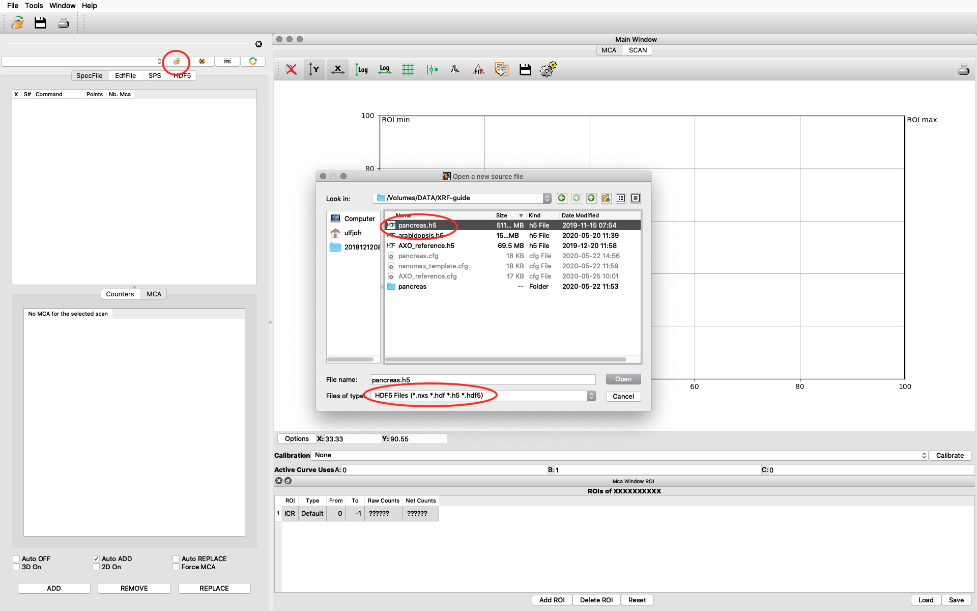
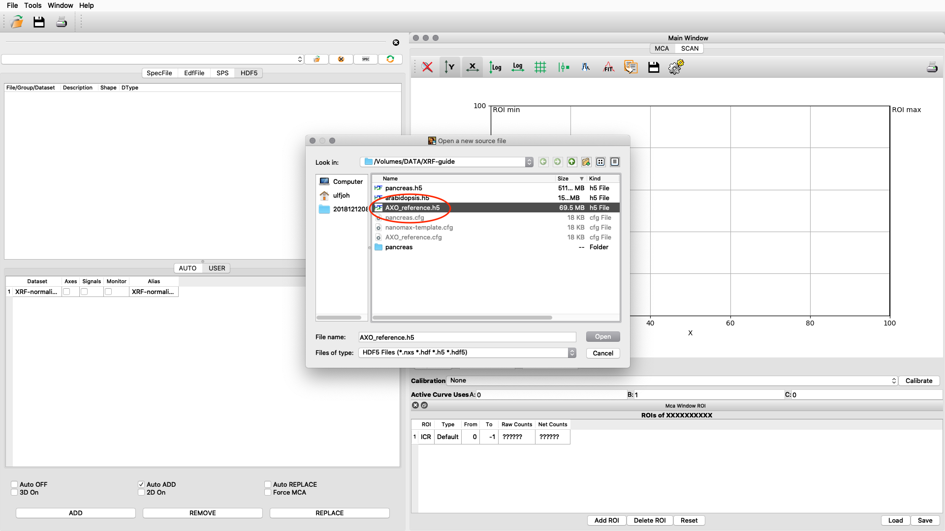
Start PyMCA. It will look like this on a MAC, similar on Windows and Linux. Click file open. Browse to your data file. Select file type HDF5. Select your file and open. In this example we open pancreas.h5.
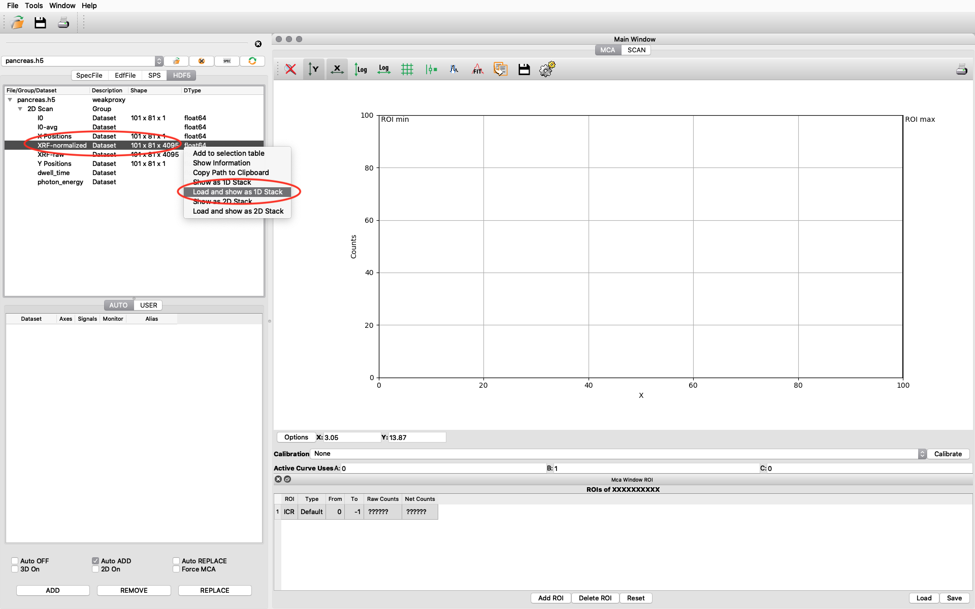
The file data structure is shown below. Select the XRF-normalized entry, right click and choose Load and show as 1D Stack. The normalized XRF data is normalized to incident photon intensity AND to 1 second acquisition time per scan point. It is important to remember the 1 second normalization in the calibration to determine absolute concentrations.
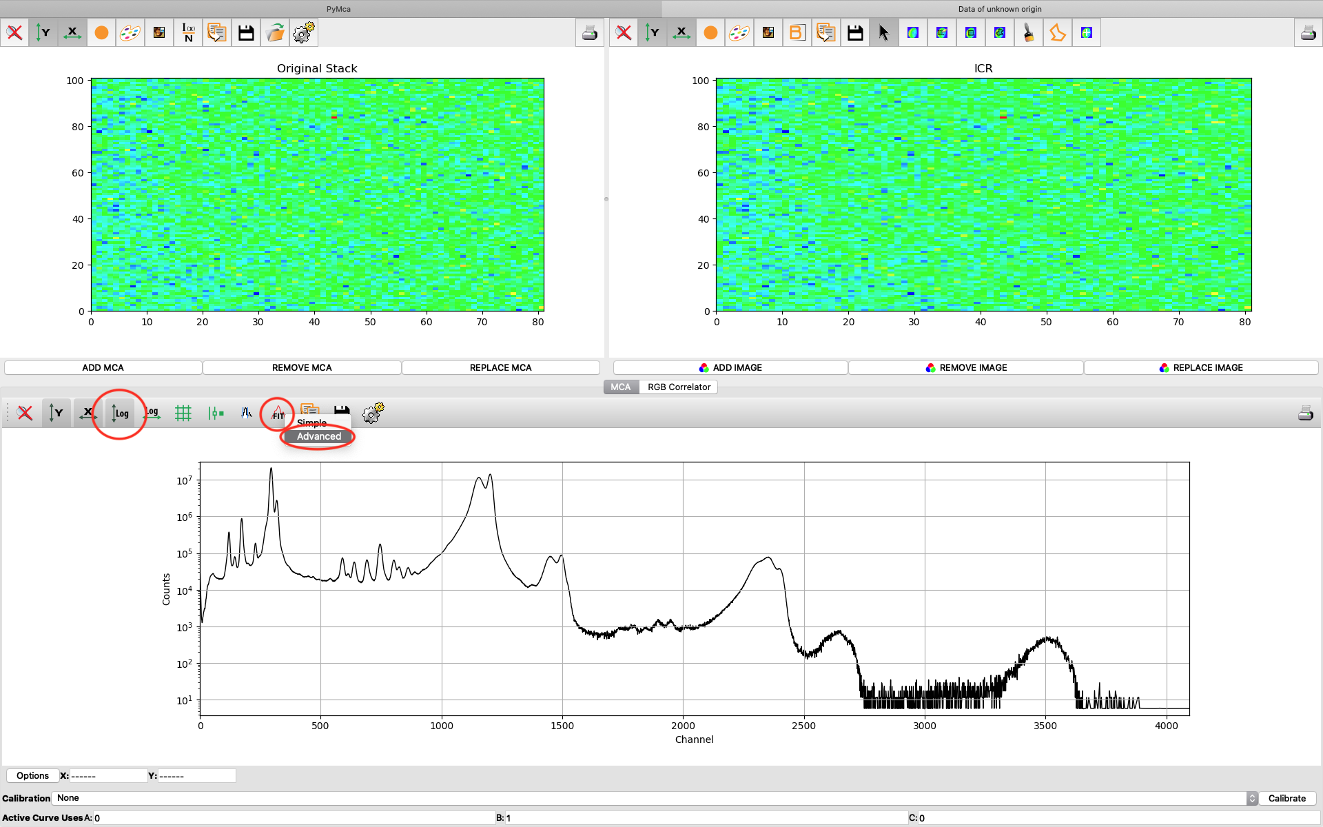
A new window opens where the summation spectrum is shown at the bottom. We will not use the two images above. With the buttons above the spectrum you can choose logarithmic y-axis. This is typically how an XRF-spectrum is displayed. In the button bar, click fit and choose advanced.
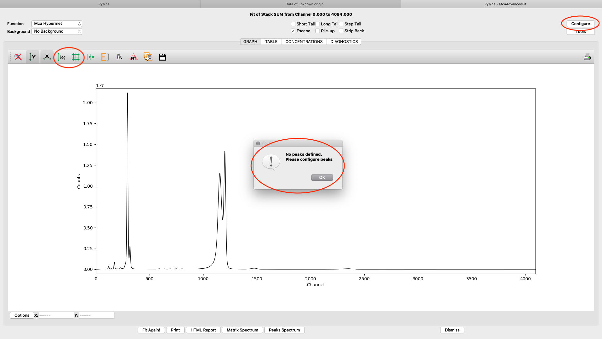
A new window with the sum spectrum opens. A dialog box says No peaks defined. Close it and select configure.
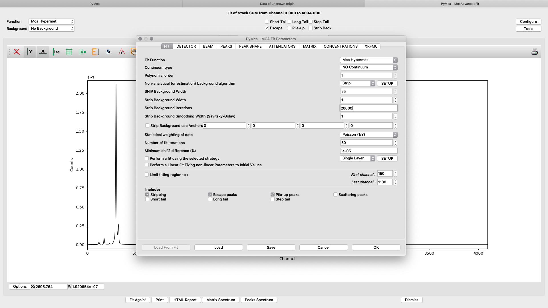
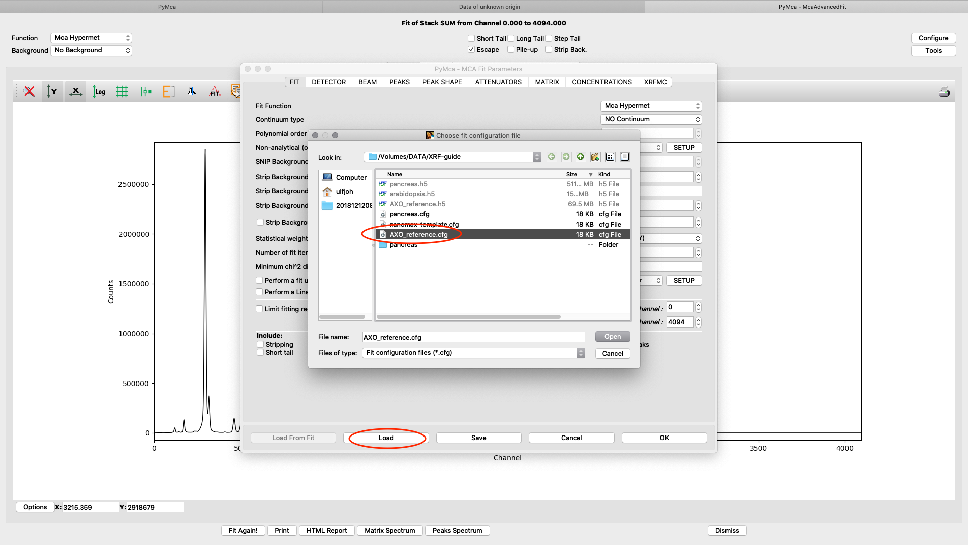
The fitting configuration dialog, with multiple tabs opens. This is where you will adjust parameters to achieve to a good spectral fit. The configuration will be used in the later elemental images creation. Instead of entering all parameters from scratch you should load a good initial configuration where several of the parameters are pre-determined. E.g. detector specific numbers, energy calibration etc. The beamline staff is normally supplying a template or an already adapted configuration file in the process/XRF_PyMCA directory.
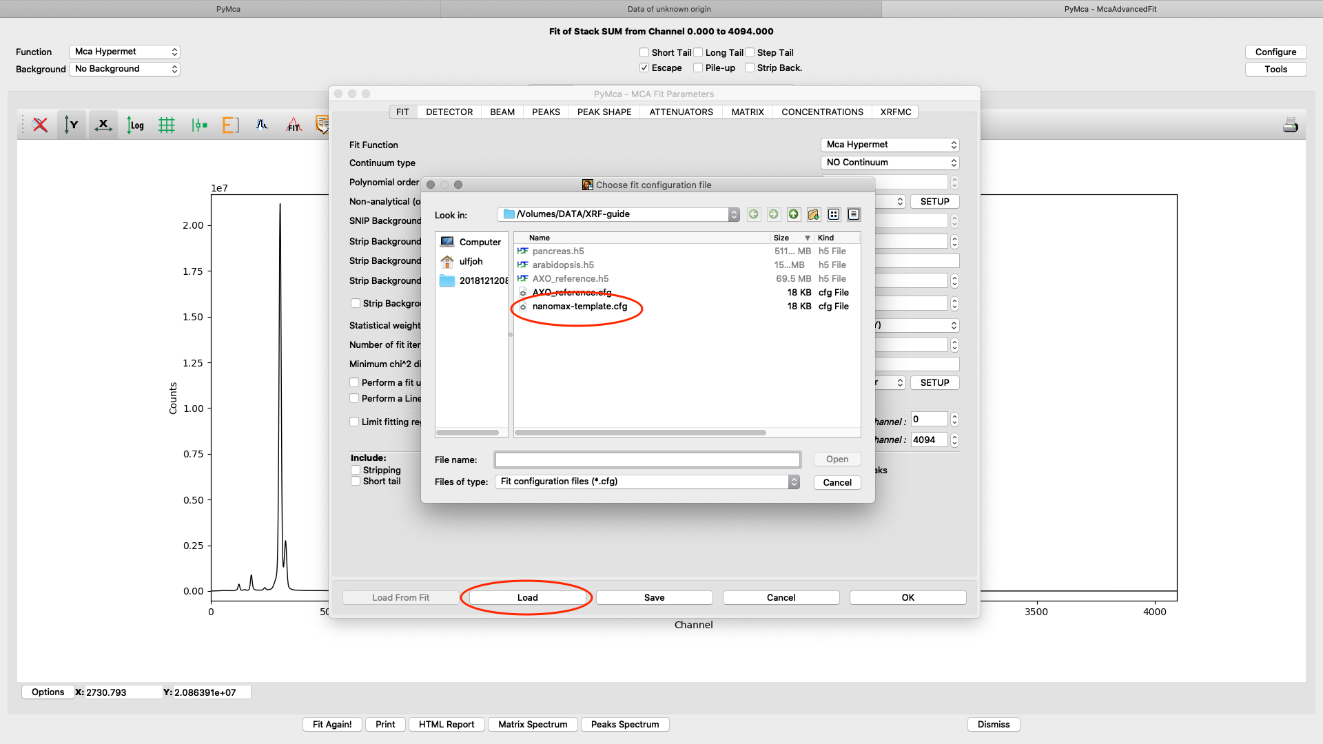
Load the template configuration file. Here we use the nanomax_template.cfg
All parameters in the configuration dialog box are updated with new values. Below are the most important ones are described.
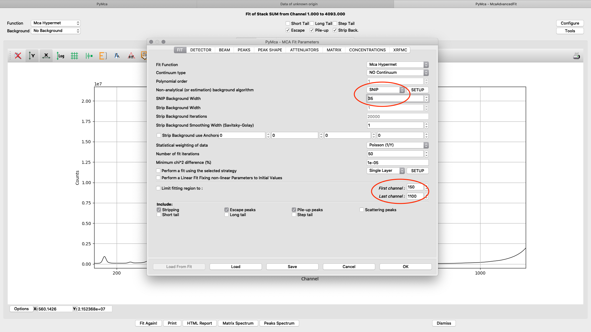
On the fit tab you can control the behavior of a smooth background with the SNIP parameter value. With the First and Last channel values you select the part of the spectrum to fit. You should select the part of the spectrum that omits low energy odd detector behavior and up to a part of the Compton and elastic scattering peak slope, normally a value of 150 works well for the low energy side. The upper limit will be determined by the used incident photon energy. In the example we are using 1100 for a photon energy of 12 keV. (one channel corresponds to 10 eV)
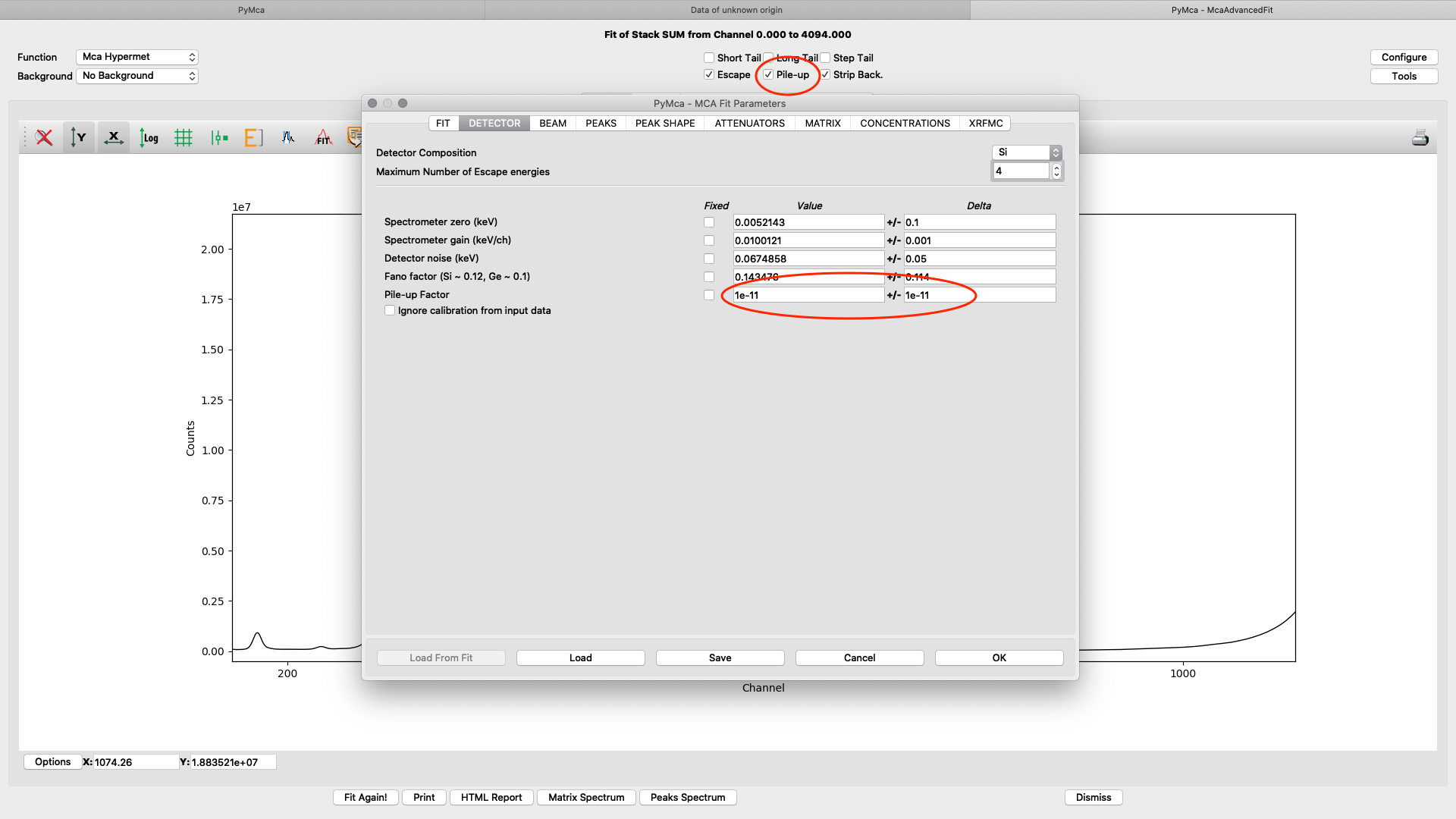
On the detector tab the pile-up parameter can need adjustments to reach to a good fit, if pile-up is selected in the fit (on the fit tab or the spectrum window). In the following example an initial number of 1E-11 for Value and Delta gives a good fit.
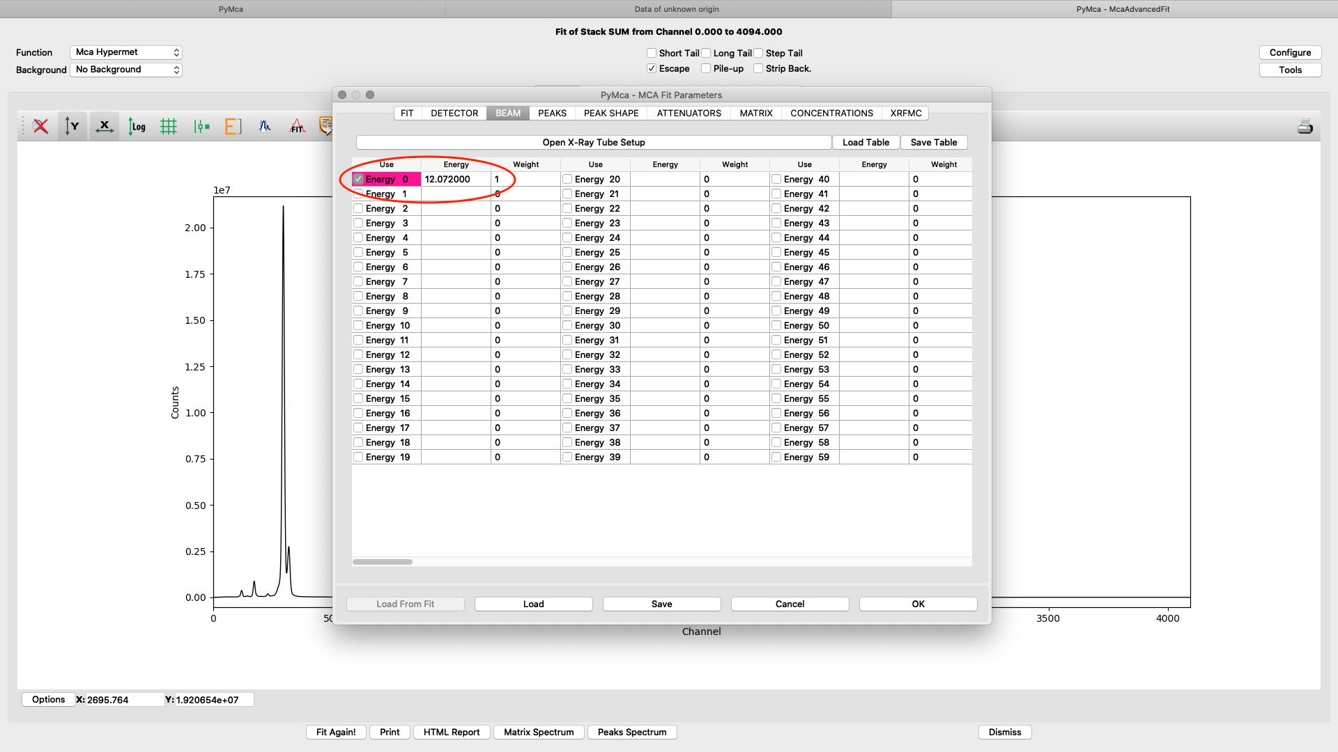
ab beam. Enter the used beamline photon energy in KeV. Make sure the box is ticked and weight is 1.
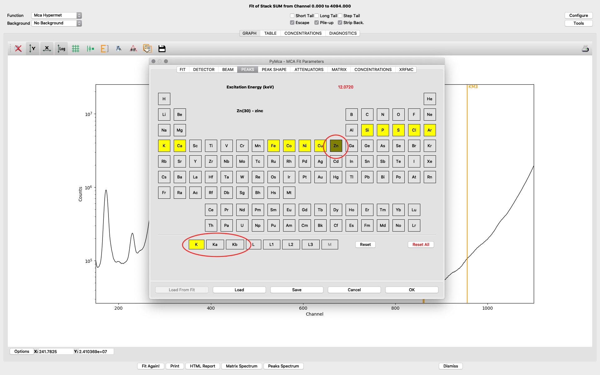
The peaks tab is where you select elements from the periodic table to include in your fit. You select an element by clicking it. Then you select the lines to include. The element and line (e.g. Zn, K-lines) turns yellow. The difference of choosing K and Ka,Kb is that K is fitted as one entity with a tabulated ratio between Ka and Kb. If you select the individually, they will be independently fitted. In most fits we use K, not the individual lines.
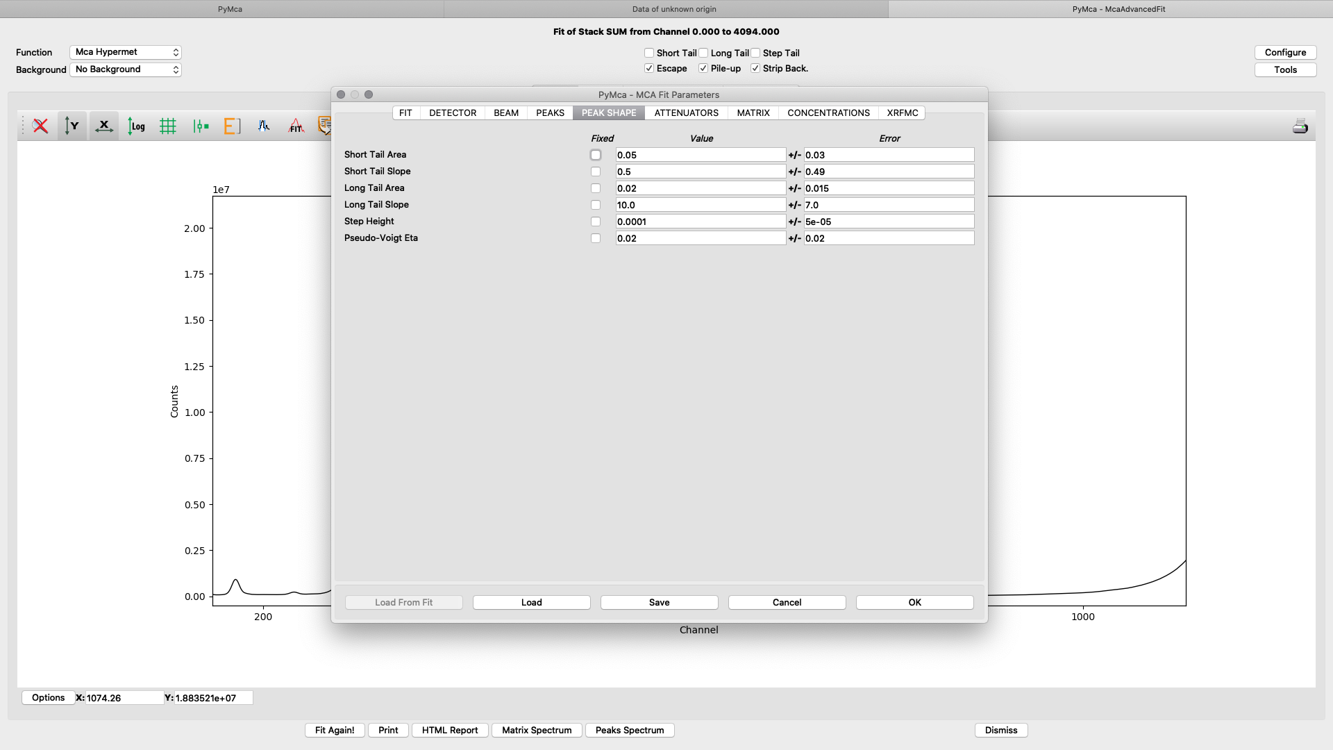
The peak shape tab is typically left with default values.
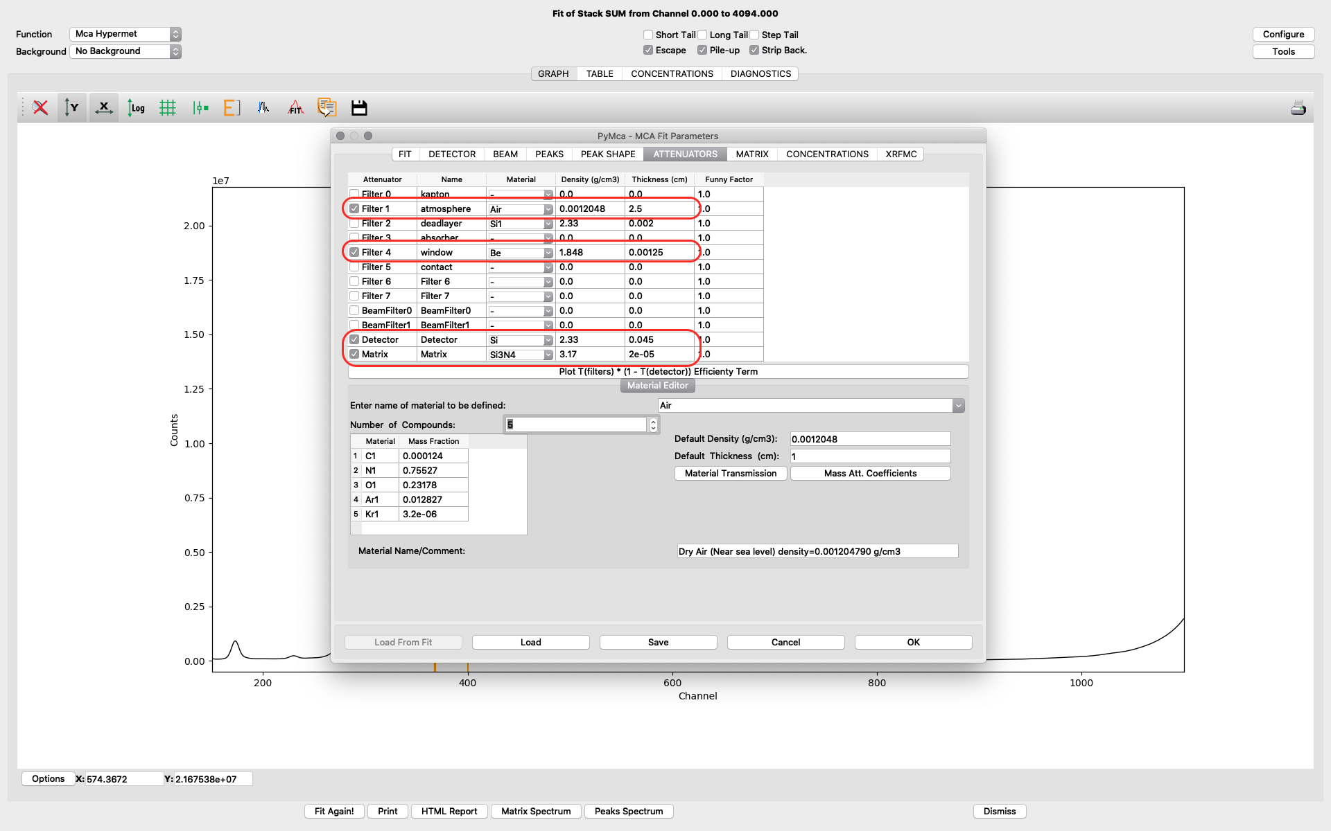
The attenuators tab. It is important to set parameters correctly on the attenuator tab to allow for correct quantification in later elemental maps creation.
Filter 1 represents the air path between the sample and the detector. Verify you have the correct thickness, corresponding to the experimental setup of your experiment. Typical value is 2-4 cm.
Filter 4 represents the thin window of the RaySpec detector at NanoMAX. The correct value is 0.00125. (12.5 um)
Detector should be selected. The thickness value should be 0.045.
In the shown example fitting, a very thin sample (< 1 um pancreas tissue) is mounted on a thin Silicon Nitride window. We have therefore defined the sample matrix to be the Si3N4 window supporting the sample. The thickness of the window is 200 nm, entered as 2e-5 cm.
For your sample condition you need to modify of the Matrix parameter. For thicker samples or layered samples, you can select Matrix as Material and further define the sample structure on the following matrix tab. See the PyMCA home page or other literature for further details on sample definition.
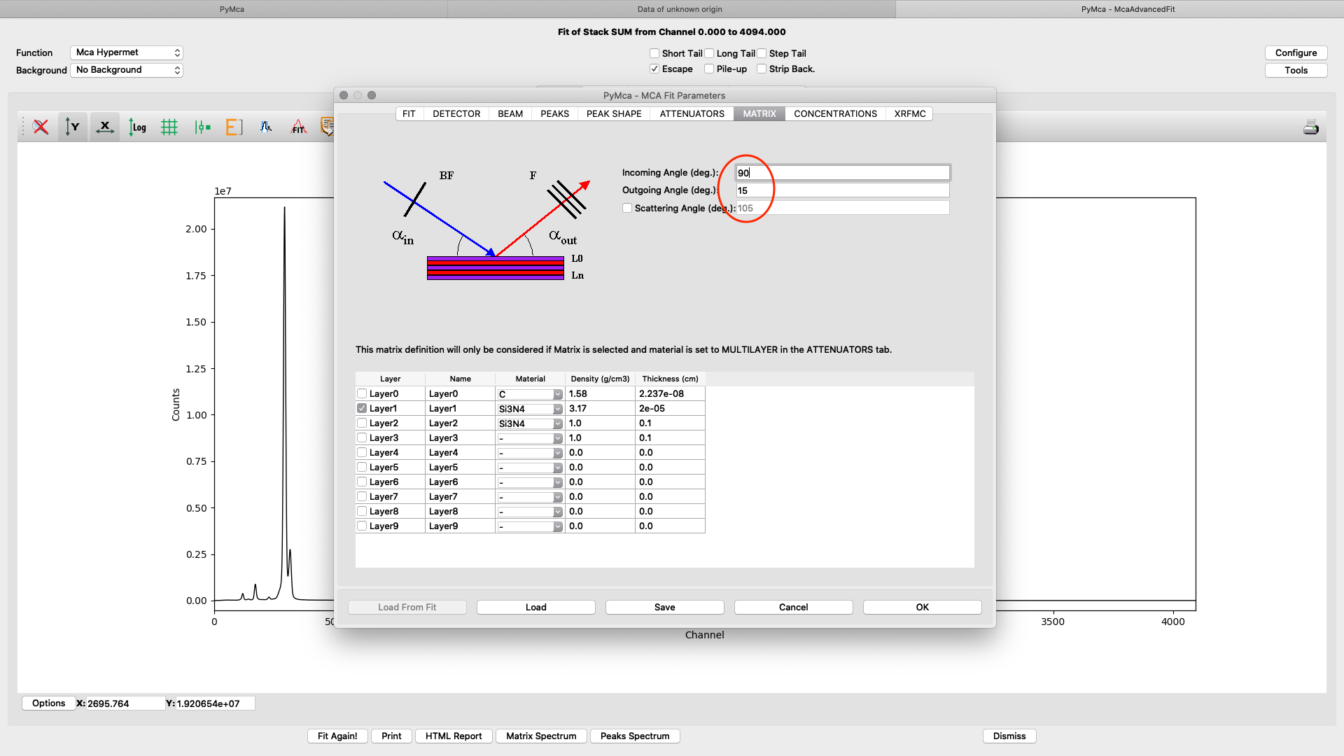
The upper part of the matrix tab defines the excitation and fluorescence beam geometry. For experiments conducted before summer 2022 the values should be 75° and 15 ° respectively, unless you used a specific setup. For later experiments the standard geometry is 90° and 15° respectively. The lower part defines layered or complicated sample compositions. This guide is not explaining how to use these options. Please read the PyMCA documentation pages.
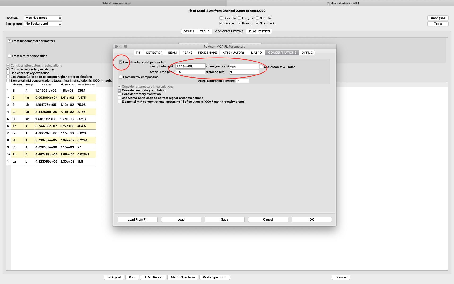
To achieve relative concentrations for comparative analysis, the parameter values on this tab are not important. They only need to be the same for all compared samples. However, if the aim is to generate elemental maps with absolute concentration values, expressed as ng/mm2, they are important. We normally use the option From fundamental parameters when analyzing thin samples. The time value should be set to one (1), since we are analyzing data normalized to 1 second. The Active area describes the acceptance of the detector. In our case the value is 0.5 cm2 for the RaySpec detector used. The distance should be the same as used for atmosphere distance in the attenuator tab plus 0.5 for internal length in the detector (2.5+0.5=3.0). If you aim at doing a data analysis with absolute elemental concentrations, the photon flux value should be determined from a reference sample. This procedure is described later. For a qualitative analysis you can have any flux number, as long as you keep it the same for all fittings.
Close the configuration dialog and do a first fit.
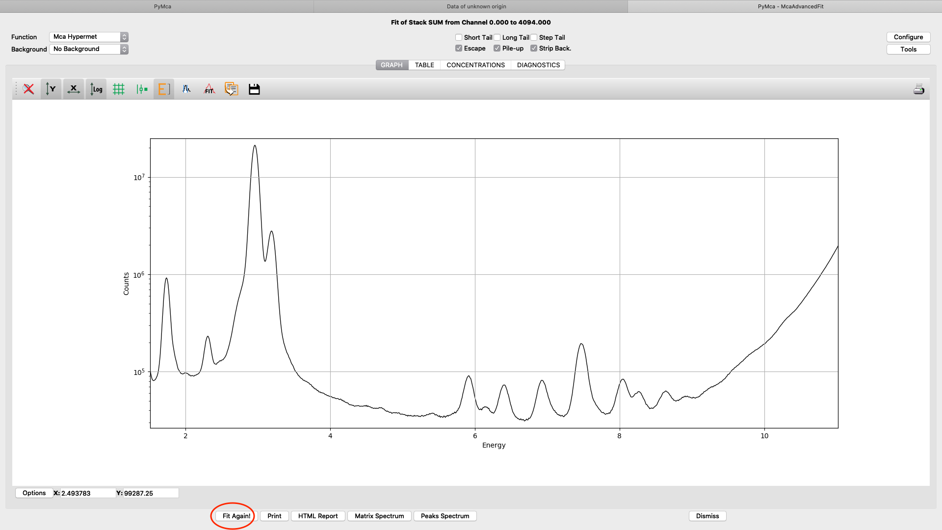
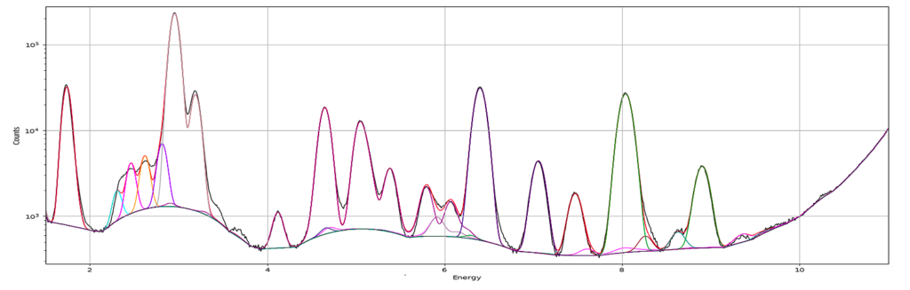
Iterate configuration parameters, mainly on the Peaks tab, to reach a good spectral fit. View the result in different ways.
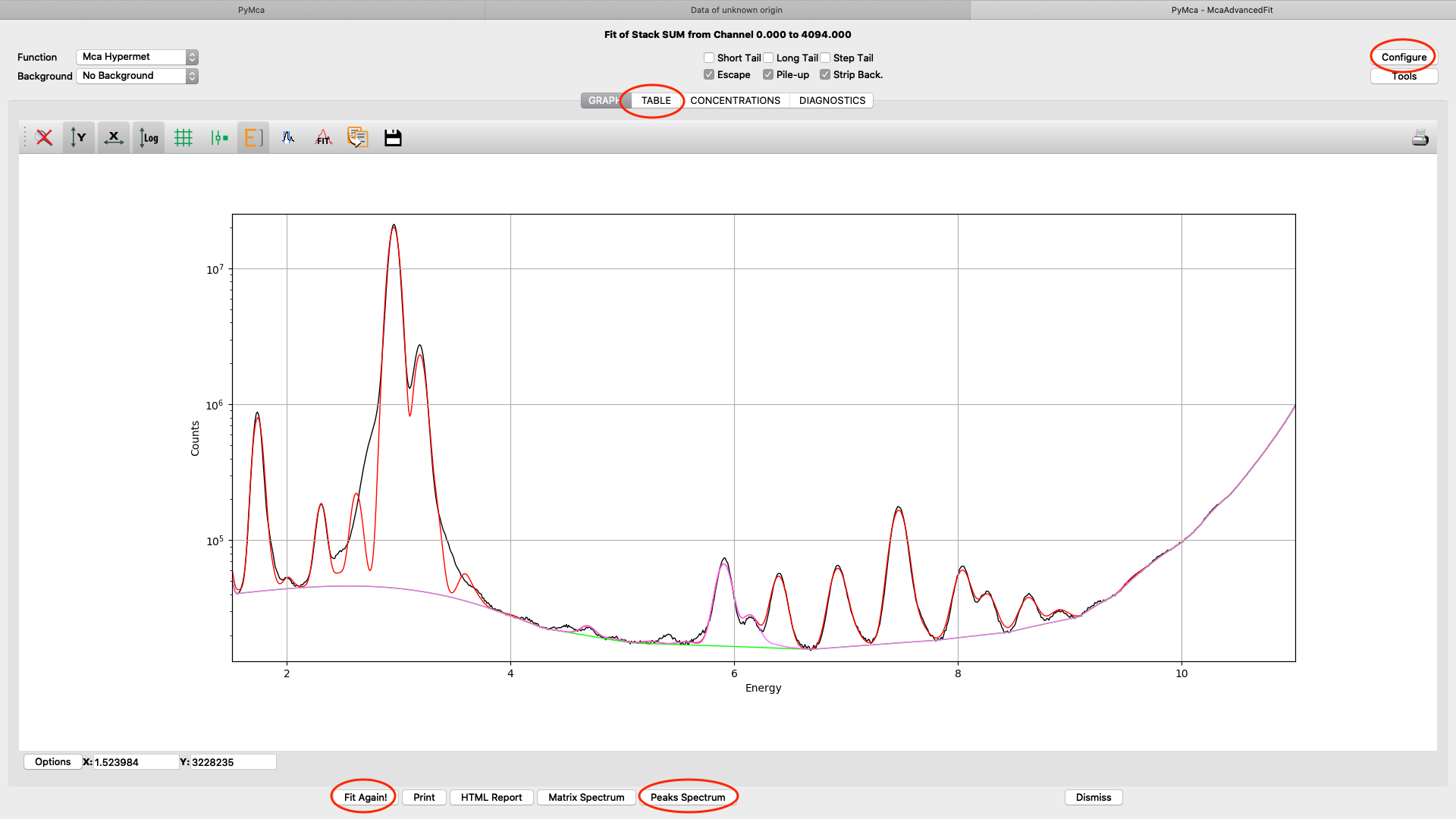
When you are satisfied with your spectral fit, open the configuration and click Load from Fit. By this you read back the optimized fit parameters into the dialog box entries. A dialog box saying “If you do not use an eponential background, …”. Since we are not using exponential background, confirm the message.
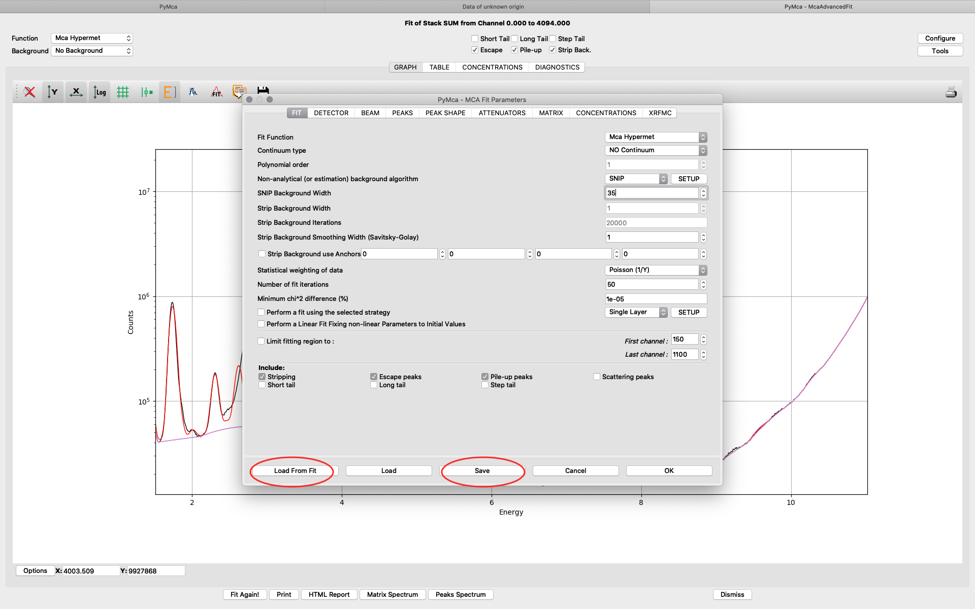
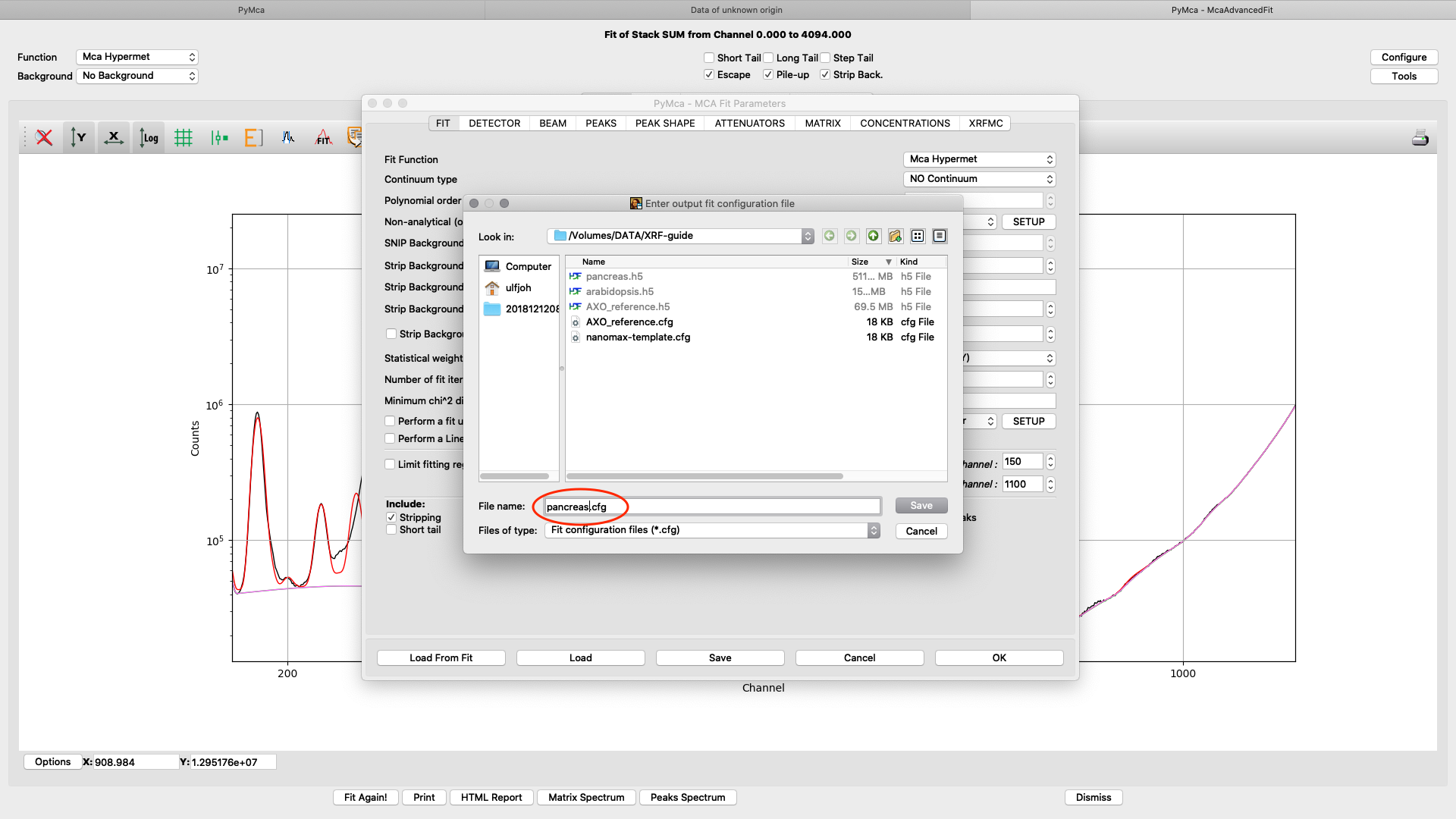
Save the configuration to a new file name (here pancreas.cfg). Close the dialog and the McaAdvancedFit window.
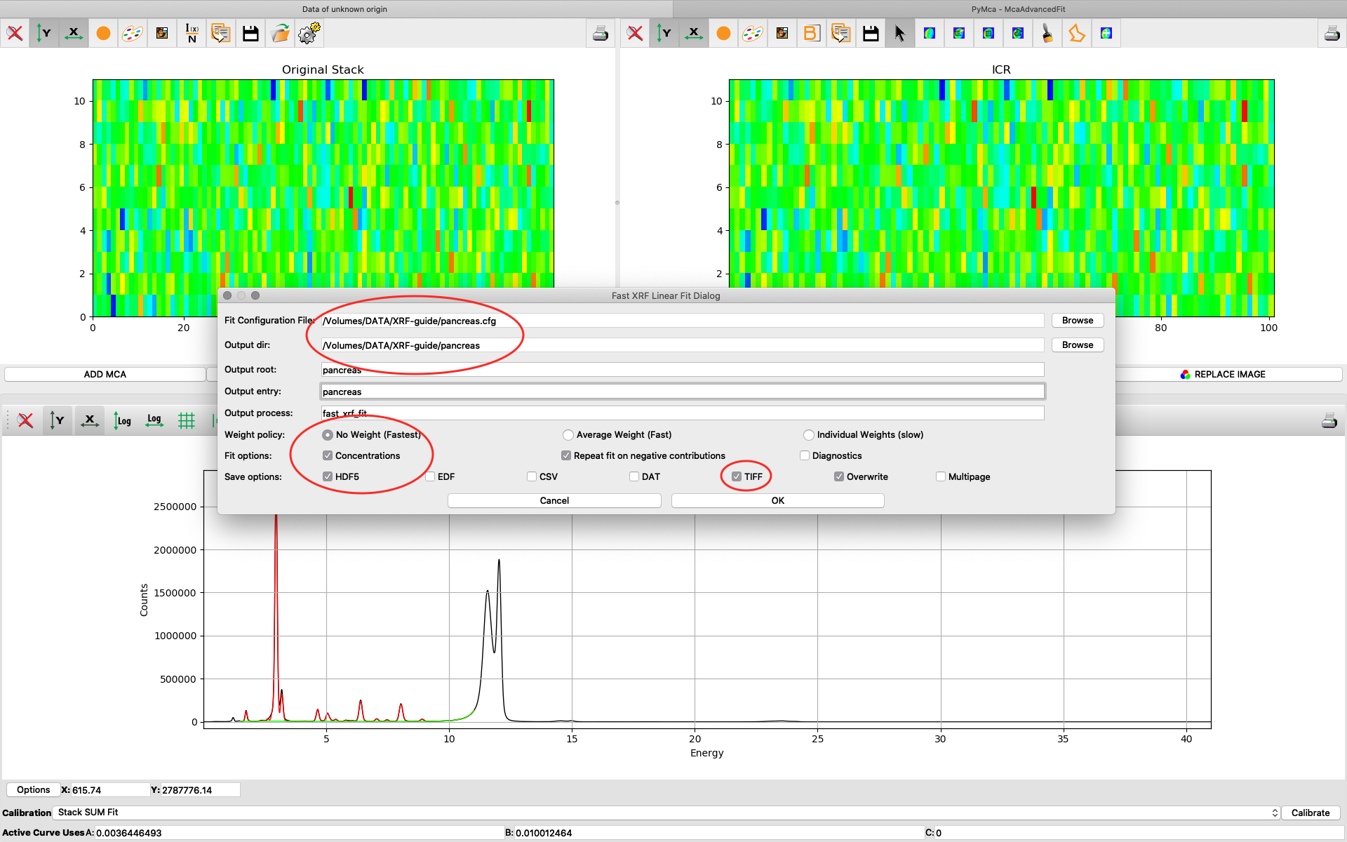
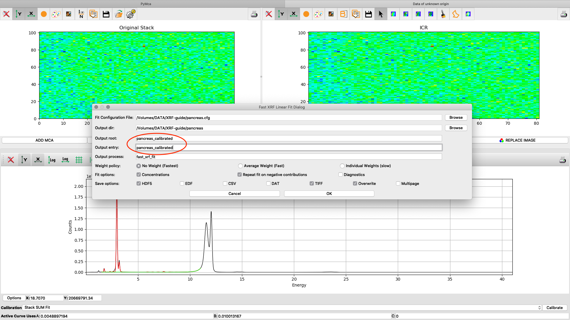
Now it is time to generate elemental maps using the saved configuration file. Open the Fast XRF Stack Fitting dialog.
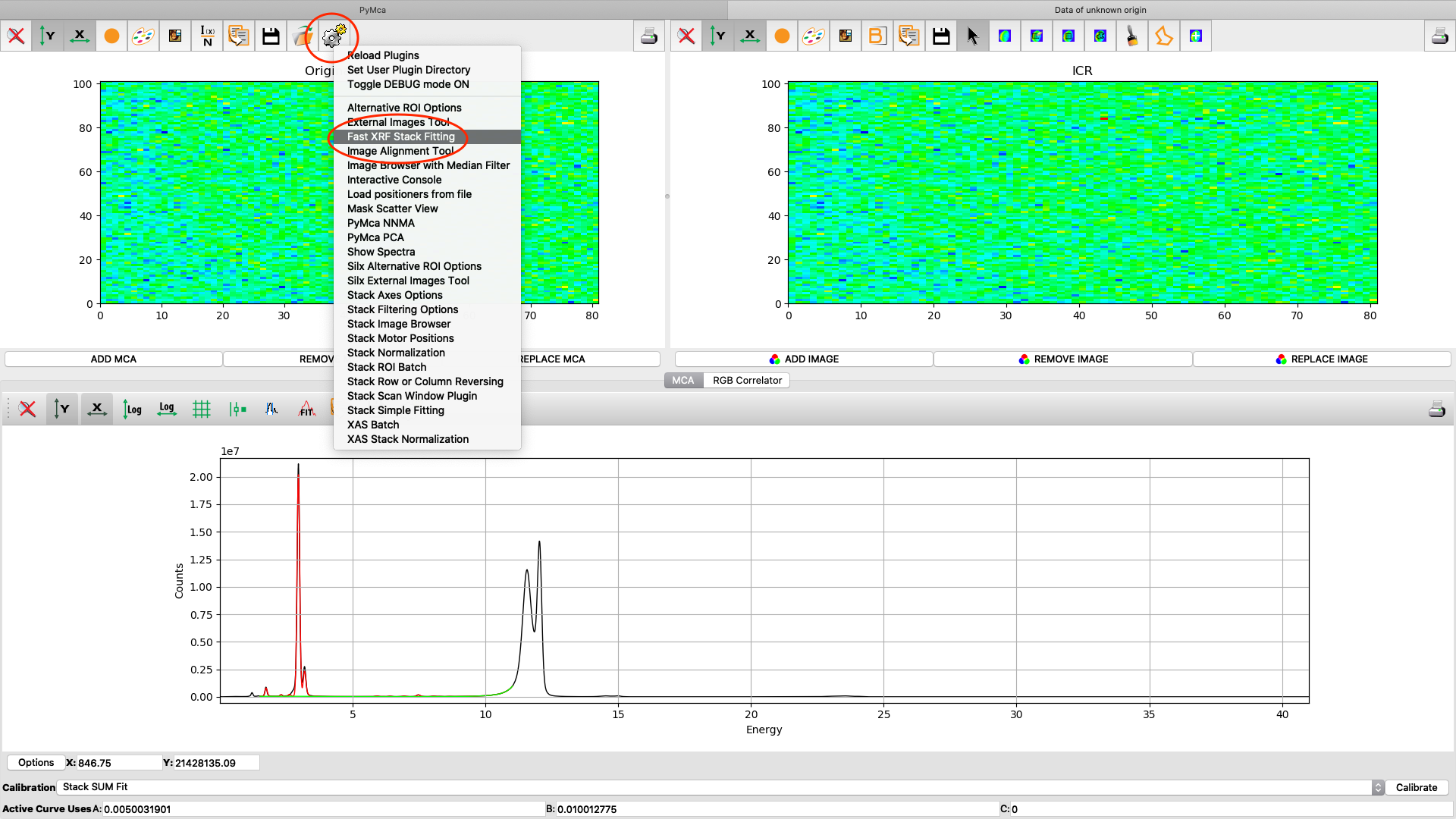
Fill in the dialog box with the optimized configuration file and a path where to place the generated files. Select options as indicated in the screenshot or other options. Normally best result is achieved by using No Weight for most samples, particularly thin and weakly fluorescing ones. An explanation of this parameter is found in the PyMCA mailing list entry https://sourceforge.net/p/pymca/mailman/message/36873045/
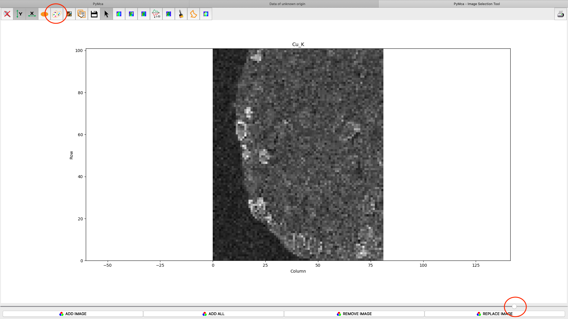
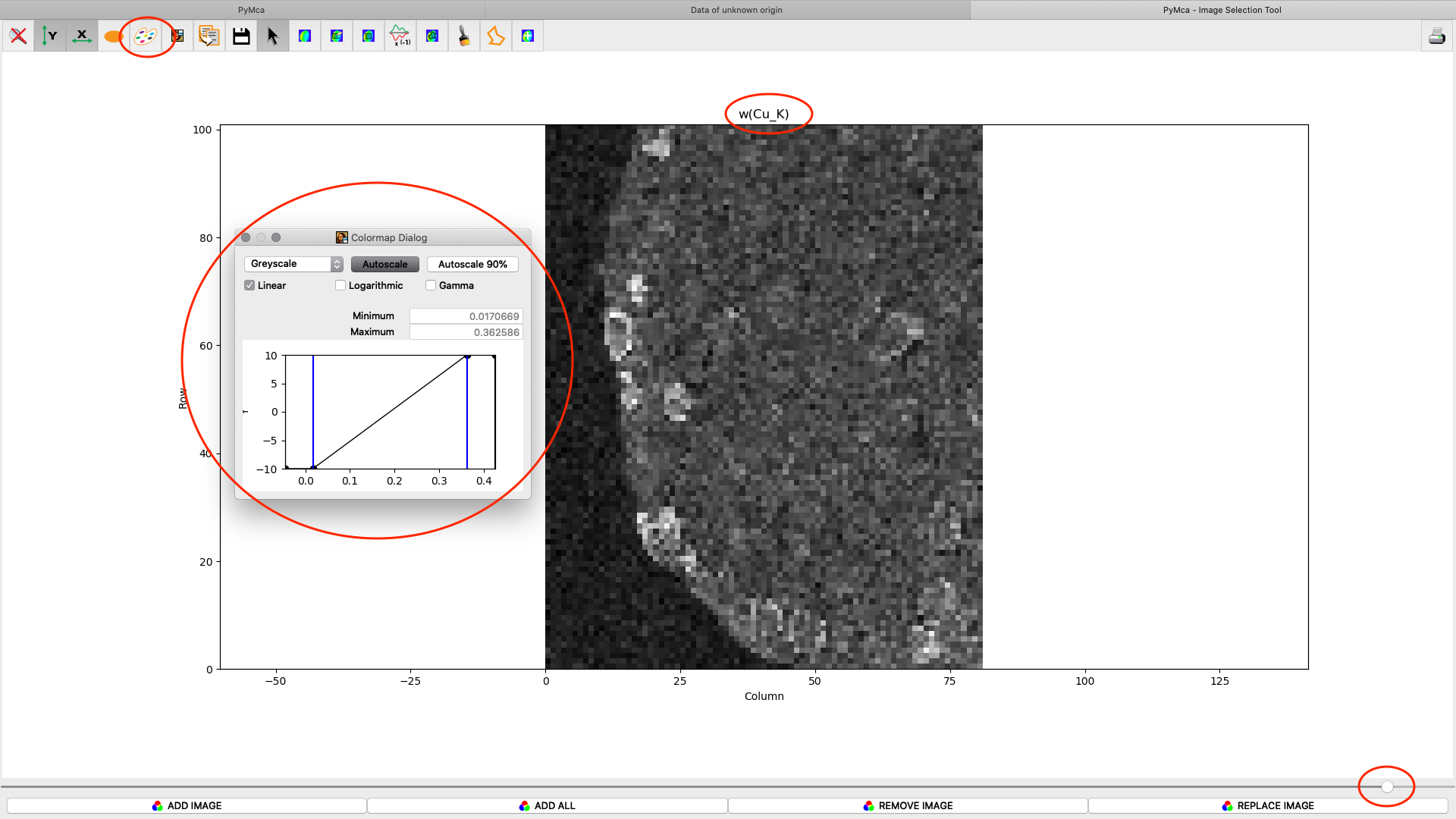
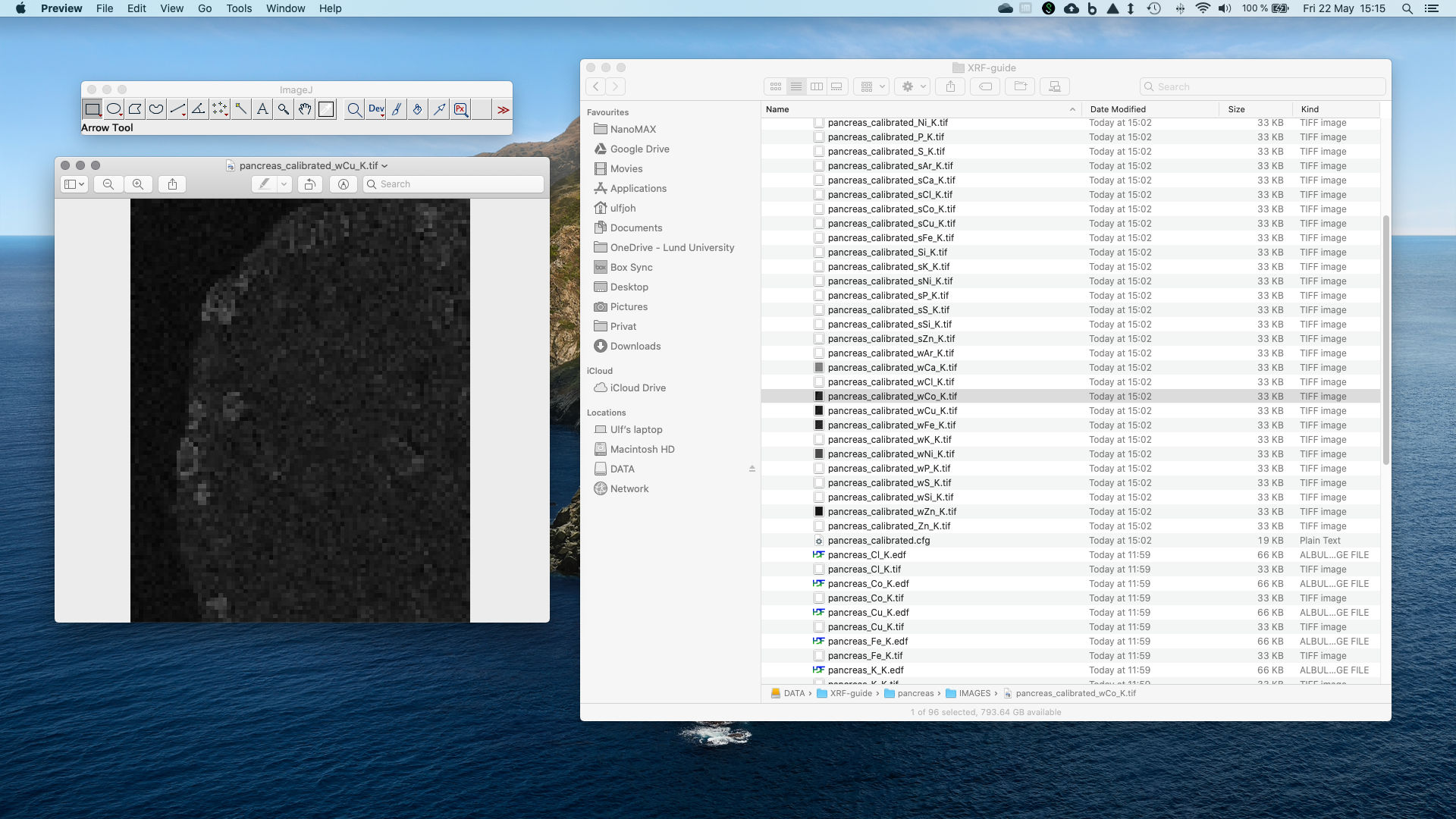
After the stack fitting procedure, a window is showing the elemental maps. A slider at the bottom is used to select element to view. Use the palette tool to set colour scheme and scaling. Images can be exported to CSV and TIFF formats. If you selected TIFF in the fitting dialog, a sub directory with TIFF files is generated. File names with _w are images with concentration values. If you have calibrated the photon flux value in the configuration file, the values in these TIFF files are ng/mm2. Otherwise the unit is arbitrary, but maps generated with the same configuration file can be compared.
Element concentrations
To analyze samples quantitatively an X-ray fluorescence reference standard is normally used. The standard we often use is a thin film sample, where several elements have been deposited on a very thing silicon nitride window. AXO Dresden: http://www.axo-dresden.de/mainframe_reference.htm
The calibration measurement must have been done with the same conditions as your samples were measured; the same photon energy, incidence angle, exit angle, distance to detector, surrounding of the sample area, etc. Calibration should be measured right before or after the sample measurement.
The standard is normally measured as an image scan but with fewer points. Load the reference scan as described earlier.
Load the AXO_reference configuration and do a spectral fit.
The fit should look similar to this. Click the concentrations view
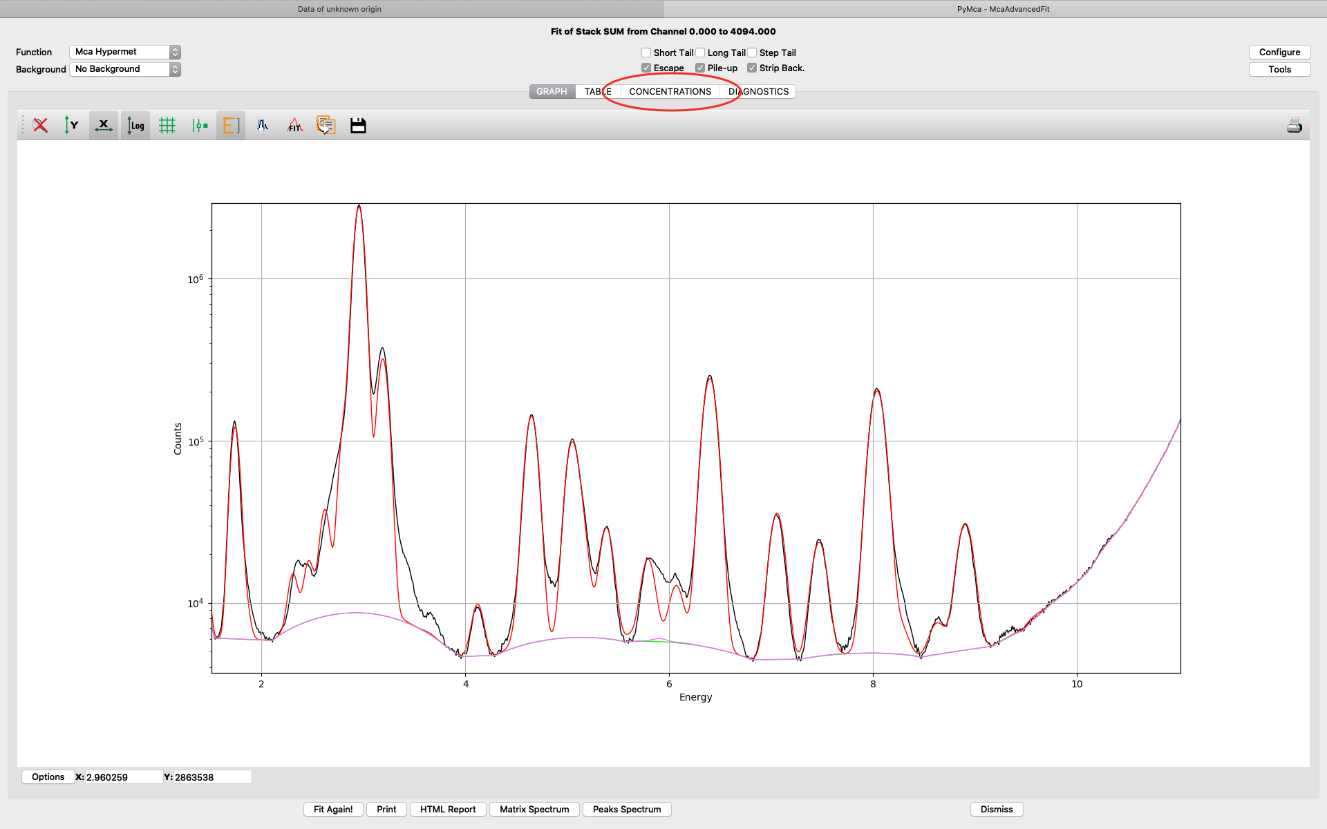
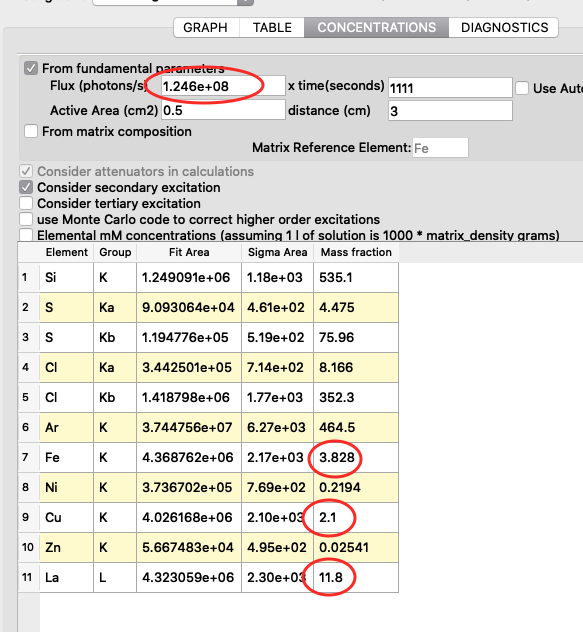
The detector active area (0.5 cm2) and the detector distance were discussed before. Use the same values as was entered for the measured samples (3 cm). X time (seconds) should be set to the number of scan points of the reference scan. In this example the refenerence standard was scanned 11 x 101 = 1111 scan points. Since data is normalized to seconds and intensity the value to enter is 1111 seconds. As you enter values in the dialog, the table of elements is updated. Adjust the photon flux value to reach mass fraction values corresponding to the real values of the reference standard. In this case photon flux has been adjusted for Cu to correspond a concentration of 2.1 ng/mm2. This is the value from the data sheet for AXO standard we use. Fe and La also correspond well to the data sheet. Note the resulting photon flux value 1.246*108. (Note, this is not the true photon flux on the sample, but only a normalization number)
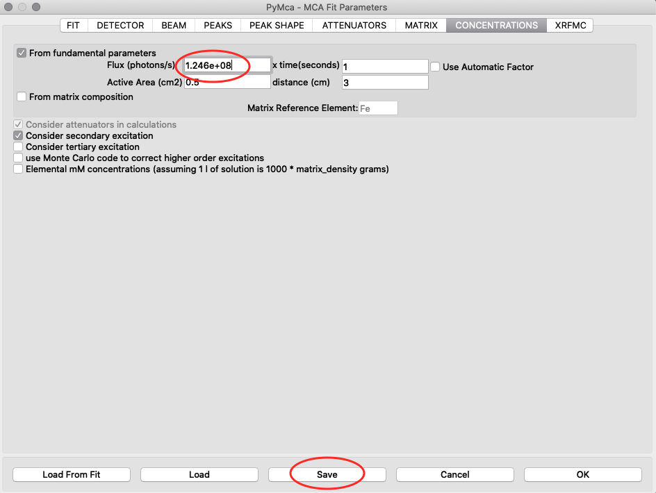
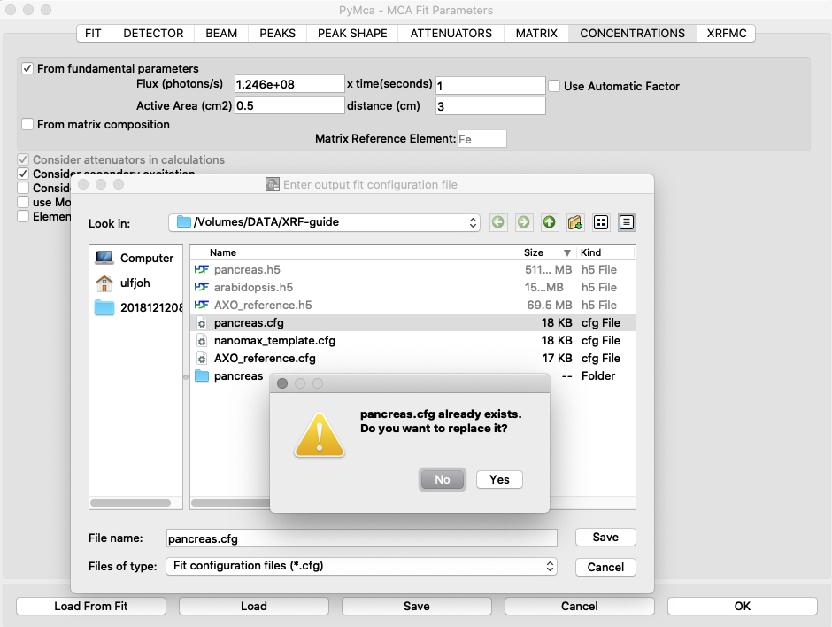
With the known photon flux value, it is time to insert the value into the configuration file for the real samples. Open the configure dialog as before, load the pancreas configuration pancreas.cfg and go to the concentrations tab. Enter the normali photon flux value, and save the configuration.
Generate new elemental maps with the calibrated configuration file. Image names containing _w are elemental maps with concentrations expressed in ng/mm2.
Three colour mapping
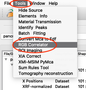
An illustrative way of showing fluorescence elemental maps, and correlation between elements is to use a three colour map. From the main PyMCA window, select
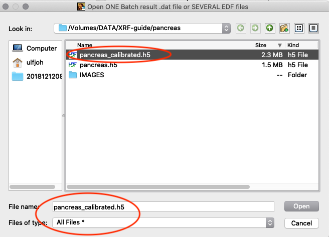
Tools/RGB-Correlator. Select the output H5 file from the stack fitting. Open the tree-structure and select plotselect.
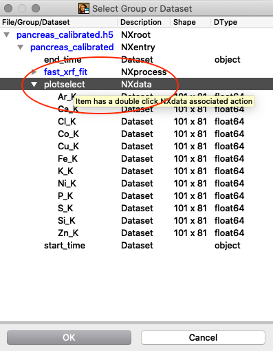
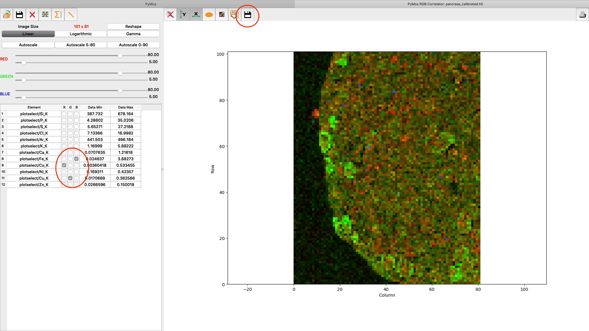
A list of elements to visualize is shown in the left panel. Map element to colour, set limits and scaling as you like. Export the image to png or jpg files. Play around with the various options.
PyMCA has many more useful features which are not described in this guide. Enjoy!
Fiji
Fiji is a free program you can use for further manipulation of your images. It can also do various analysis of the exported tiff files in the output directory.
The download is found here: https://imagej.net/Fiji
(Ulf Johansson, NanoMAX beamline scientist, 2022-12-08)