Data handling and processing at MX

The image files from the Eiger2 and Jungfrau detectors are written out in the NeXus format, using the HDF5 data convention as a container. Each h5 container stores up to 1000 images. For each data set a master file is written containing experimental and instrumentation metadata that complies with the Gold Standard for macromolecular crystallography diffraction data. The files are stored in a directory of the form /data/visitors/’beamline’/’proposal’/’date’/raw/’yourprotein’/’yourprotein-yourcrystal’. For proprietary proposals, the path is the same, but replacing ‘visitors’ with ‘proprietary’. The /data/visitors and /data/proprietary directories are mounted on all the MAX IV computers available to users.

Important: don’t change the file names or paths, which might break the internal data-links and also causes failure of most software.

During the experiment, the data are available on the high speed local storage at MAX IV.  After that, non-proprietary data are archived. Note that although the data are on a separate location after archiving, you can still use the the same path (displayed in EXI) to access the data. The data can be accessed for transfer via Globus or sftp. They can be made public via SciCat. Further offline processing can be carried out remotely at LUNARC or, for small jobs, on the MAX IV offline HPC cluster.

As soon as a data set has been collected and written to the local disk, MXCuBE3 launches several automated data processing pipelines. fast_dp and EDNA produce very fast results for rapid feedback on data quality, while autoPROC and DIALS runs significantly slower; autoPROC performs anisotropy analysis which results in better data in some cases. The output files of the automated processing are stored under the ‘/data/visitors/’beamline’/’proposal’/’date’/process’ subdirectory (or  ‘/data/proprietary/’beamline’/’proposal’/’date’/process’ for proprietary proposals) , but you can also inspect the results in EXI running on a remote browser and download them directly to your own computer.

Since 2026, MicroMAX also does autoprocessing of serial crystallography data. See the section Processing SSX data below.

You can see images as they are being collected with either ALBULA or Adxv. Click the Albula Autoload or adxv autoload icon on the beamline desktop to launch your prefered program in monitoring mode.

A useful feature of Adxv  is that it can add frames together, a useful feature to assess visually the quality of the diffraction for thin phi sliced data. Use the “slabs” box to set the number of images to add together; 5-10 is a good choice for data collected in 0.1 degree frames.

Adxv can also be run offline via a script from the command line on the biomax-remote server and the beamline workstations. To load a dataset, type:
adxv_eiger xxxx_master.h5
The adxv_eiger wrapper will read all the necessary metadata information in the master file supplied. When changing to a new dataset, launch the same command from the terminal instead of loading the dataset directly in the Adxv GUI (otherwise it uses the metadata information from the previous dataset).

Users can process the data in the ‘process’ subfolder in their session directory in the /data/visitors/biomax  or /data/visitors/micromax area.
For manual data processing during or after the experiment we recommend use of the PReSTO platform, available to general non industry users on the MAX IV HPC clusters. During the beamtime, users can log in to the so called online HPC cluster. After the beamtime, users can log in remotely to the offline HPC cluster.

To log in to the online cluster (during beamtime, from the beamline machines or from remote-biomax):

• Click on Applications (first item in the top panel of the desktop).
• Hover over the Internet menu and select the ThinLinc Client application.
• Type clu0-fe-2 or clu0-fe-3 as the server, your username and your password and the return key.
• By default, the ThinLinc desktop will be set to full screen mode. You can use the F8 key to exit this.
• When you finish your work, please log out (click on the ‘username’ menu to the right of the top panel and select “Log out”. If you do not log out, your session will keep on running indefinitely.

To log in remotely from outside MAX IV to the  “offline” cluster (offline-fe1), users need to download and install in their home computer the Pulse Secure software to establish a VPN connection to MAX IV and the Thinlinc client (remote desktop) to log in to the HPC front end computer.

The offline cluster has fewer nodes than the online cluster, but otherwise the configuration is similar. The /data disk is mounted on both clusters, as well as the home disk. For more help, see IT environment at BioMAX.

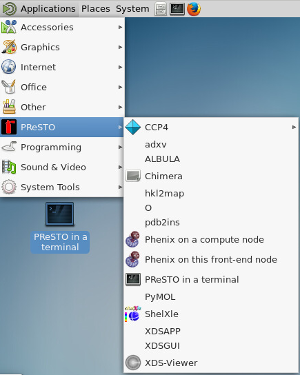
Once you have logged in to the appropriate HPC with ThinLinc, the easiest way to launch a PReSTO ready terminal is through the thinlinc client “Applications” menu.

It is possible to run jobs from a terminal window, but please do not use run resource intensive jobs on the front end. Use the compute nodes instead, either with the SLURMS sbatch command or in interactive mode:

1. open a terminal
2. Type: interactive -c 'n-of-CPUs' -t 'time'. For example, interactive -c 10 -t 01:00:00 will give you 10 CPUs for one hour.

See also HPC Basics.

Logout after using your session to release resources.

The next sections provide information to run some supported packages from PReSTO on the MAX IV cluster. To fully explore the capabilities of the software and job submission in the cluster (important if you are planning to go beyond data reduction and run longer jobs) please refer to the individual programs documentation and the PReSTO help pages. The entire list of software available through PReSTO is listed here.

XDS

XDSAPP3:

• Open the GUI: Applications → PreSTO → XDSAPP3. (the old XDSAPP does not work for data collected after February 2022)
• Allocate the number of cores and the time for the job (we suggest the maximum number of cores available and 1 hour). If you cannot get the GUI to open, it can be because the nodes are very busy; try allocating fewer cores to the job (eg, 20 instead of 24).
• Go to the Settings tab and select the location of your output directory. You must specify a directory in the ‘process’ subdirectory of your proposal or in your home area; by default, the program will attempt to create a subdirectory will be created in the directory where the input data are. This fails, as the data directories are write-protected.
• Load the master file of the data set to process. You need to choose the directory where the data are located first, then select the master file. This will populate all the fields in the “Settings” tab, used to generate the input XDS.INP file.
• You can choose whether to run the different tasks one by one or run them all as a supertask by clicking “Do all”.
• To view a graphical display of the results of the INTEGRATE and CORRECT steps and the dataset statistics, use the corresponding tabs.

XDSGUI:

• Open the GUI: Applications → PreSTO → XDSGUI.
• Allocate the number of cores for the job and the time (we suggest the maximum number of cores and 1 hour).
• On the projects TAB, select the directory where you want to store the processing results; create the directory first from a terminal if it does not exist. By default the result files will be written to the same directory as the images.
• On the Frame tab, load the master file of the data set to process and then generate the XDS.INP file.
• Edit the XDS.INP file to insert the line
  LIB= /sw/pkg/presto/software/Durin/2019v1-foss-2019b-6/lib/durin-plugin.so
  For fast processing we also recommend defining the number of jobs and number of processors in the input. The product of the two numbers should be equal to or less than twice the total number of cores allocated. Eg. on the offline cluster, insert the two following lines:

MAXIMUM_NUMBER_OF_JOBS= 5
MAXIMUM_NUMBER_OF_PROCESSORS= 8

• Save the input and click on Run XDS to start the job.

Xia2

Use an interactive node to run Xia2: Open a terminal in the thinlinc client, eg, from the Applications -> System Tools menu and load the DIALS module:
interactive --exclusive -t 01:00:00
module load gopresto DIALS

• As suggested in the example, one hour (01:00:00) is usually long enough to process the data set. For large data sets with many reflections, a longer time may be required.
• You can tell if you have obtained a data processing node by typing “hostname” in the window. The output will be cnXX, with XX being the node number. If you cannot get a node (perhaps because the cluster is very busy) try requesting fewer cores, for example:
  interactive -c 12 -t 01:00:00
  That will book only 12 cores.
• Change the directory to where you want to store the output files.
• We recommend using the dials pipeline using the command: ‘xia2 pipeline=dials image=/data/visitors/biomax/…/’path_to_master’.h5′. You can also run Xia2 to run XDS based pipelines, however running XDS directly seems to be more advantageous in that case. Type ‘xia2’ for help using the program.
• If the job finishes earlier than expected, type “exit” to release the node.

An alternative way to run DIALS is through the CCP4i2 interface (accessed through Applications → PreSTO → CCP4 → CCP4 Interface 2). Create a new project from the Project tab if necessary, and then, click on the Task menu and select Integrate X-ray images, and DIALS. When the software opens the DIALS interface, follow the screen instructions.

autoPROC

Use an interactive node to run autoPROC: Open a terminal from the Applications -> System Tools menu and load the autoPROC module:
interactive --exclusive -t 01:00:00
module load gopresto autoPROC

• As suggested in the example, one hour (01:00:00) is usually long enough to process the data set. For large data sets with many reflections, a longer time may be required.
• You can tell if you have obtained a data processing node by typing “hostname” in the window. The output will be cnXX, with XX being the node number.
• Go to the directory where you wish to store the data and start autoPROC from the command line:process -h5 /'pathto masterfile_master'.h5 autoPROC_XdsKeyword_MAXIMUM_NUMBER_OF_JOBS=5 autoPROC_XdsKeyword_MAXIMUM_NUMBER_OF_PROCESSORS=8
  Make sure that the number of jobs times the number of processors does not exceed the resources of the node, otherwise the job will fail.
• If the job finishes earlier than expected, type “exit” to release the node.

CrystFEL

PReSTO includes the program CrystFEL and the CrystFEL GUI for processing SSX data using either fixed target or injector based sample delivery.

To launch the GUI, use the command

module load gopresto CrystFEL
crystfel

Consult Thomas White guide at www.desy.de/~twhite/crystfel/tutorial.html to learn how to use the GUI.

The configuration files from the autoprocessing ssx_workflows described  in the Processing SSX data  can  be used as a starting point for manual reprocessing. The configuration files are located in:

/data/visitors/micromax/<proposal_number>/<date>/process/<protein_acronym>/<protein_acronym>-<sample_name>/all

Further advice

• Please see some of the scripts written by PReSTO developers for data processing on the MAX IV HPC clusters. Prior to running native.script or anomalous.script, the output directory must be created.
• This is the pipeline that appears to generate the best results to date:
  1. Process with XDSAPP3 to 0.3-0.4 Å higher resolution than XDSAPP3 suggests by default.
  2. Use the output XDS_ASCII.HKL as input for the STARANISO server.The resulting anisotropic dataset will be better than standard autoPROC run.
• Try out DIALS, since this software is undergoing continuous improvement.

Autoprocessing of serial crystallography data is performed using an in-house developed workflow named ssx_workflows, based on CrystFEL

Autoprocessing results are stored one of two subdirectories of 

/data/visitors/micromax/<proposal_number>/<date>/process/<protein_acronym>/<protein_acronym>-<sample_name>/

named:

• <protein_acronym>-<sample_name>_<run_number>_crystfel for Jungfrau data
• crystfel_<protein_acronym>-<sample_name>_<run_number>for Eiger data.

Unit-cell parameters and space group are provided through the MXCuBE interface. When these parameters are not provided, the workflows are configured automatically, but must be triggered manually.

Workflow settings and behaviour are controlled through template files and can be discussed with staff before and during beamtime.

A typical autoprocessing strategy consists of the following steps:

1. Peak finding and parameter optimization

For each unique combination of <proposal_number>, <date>, and <protein_acronym>, spot-finding parameters for peakfinder8 are optimised by maximising the indexing rate over a 3D parameter grid using a subset of the data.

The subset size and grid parameters are configurable. The indexing algorithm used at this stage is typically mosflm, although xgandalf can also be used.

The parameter set that yields the highest indexing rate is selected. If other parameter sets achieve the same maximum indexing rate, the setting with the shortest runtime is selected.

If the maximum indexing rate exceeds a configurable threshold, the parameters are written to:

/data/visitors/micromax/<proposal_number>/<date>/process/<protein_acronym>/pf8_paras.json

and are subsequently used for all processing sharing the same <proposal_number>, <date>, and <protein_acronym>.

2. Beam position optimization

For each detector run, a subset of the data is processed using the optimised peakfinder8 parameters and, typically, mosflm as the indexer in order to optimise the beam position.

• If CrystFEL version 0.11.0 or later is used (recommended), the beam position is refined using millepede.
• If CrystFEL version 0.10.x is used, the beam-centre shift is estimated from the average shift of individual patterns determined by indexamajig.

3. Full data processing

The complete dataset is processed using the optimised peakfinder8 parameters and beam position. At this stage, the workflow is typically configured to use xgandalf as the indexing algorithm.

Unless agreed otherwise, ssx_workflows is configured to perform steps 1-3 automatically and without user intervention.

Monitoring processing quality

Users are recommended to inspect unit-cell distribution plots located in subdirectories of the processing directories:

ssx_wfs_pf8/ssx_wf_output_pf8spots_xgandalf_1/uc_distributions.png

and workflow reports located at:

ssx_wfs_pf8/report.html

Monitoring indexing rates and unit-cell distribution shapes enables early detection of issues such as low indexing rates or distorted unit-cell distributions.

Time-resolved experiments

In time-resolved experiments, data are processed in time classes. Per-class stream files and unit-cell distribution plots are generated automatically.

Reprocessing data

Although reprocessing is typically not required, ssx_workflows can also be used for data reprocessing. If reprocessing at MAX IV, please see the Manual data reduction section above.

The configuration files are located in:

/data/visitors/micromax/<proposal_number>/<date>/process/<protein_acronym>/<protein_acronym>-<sample_name>/all

Users may wish to reprocess data if an error in detector distance is suspected. In this case, ssx_workflows can be configured to perform a detector-distance scan and optimise the detector distance by minimising the widths of the unit-cell parameter distributions.

Reprocessing may also be required if the final unit cell obtained from Gaussian fitting of the unit-cell distributions differs significantly from the target unit cell provided by the user.

Merging Serial Crystallography data

Scripts for downstream data processing are located in:

/data/visitors/micromax/<proposal_number>/<date>/process/<protein_acronym>/<protein_acronym>-<sample_name>/all/merge

These scripts support:

• indexing ambiguity resolution using ambigator (only for space groups exhibiting indexing ambiguity)
• data merging using partialator
• merging statistics calculation
• conversion from HKL to MTZ format
• reindexing using pointless with a reference model (only for space groups exhibiting indexing ambiguity)
• map calculation using dimple (requires a PDB model)
• difference map calculation (requires a PDB model)
• extrapolated map calculation (requires a PDB model)

To display usage instructions, run:

./<script_name>.sh --help Creating a merged stream file

cd /data/visitors/micromax/<proposal_number>/<date>/process/<protein_acronym>/<protein_acronym>-<sample_name>/all/merge
rm -f all.stream
for i in ../../*crystfel/ssx_wfs_pf8/ssx_wf_output_pf8spots_xgandalf_1/processing.stream
do
    echo ${i}
    cat $i >> all.stream
done

cd /data/visitors/micromax/<proposal_number>/<date>/process/<protein_acronym>/<protein_acronym>-<sample_name>/all/merge
for k in {0..9}
do
    echo ${k}
    rm -f class_${k}.stream
    for i in ../../*crystfel/ssx_wfs_pf8/ssx_wf_output_pf8spots_xgandalf_1/class_${k}.stream
    do
        echo ${i}
        cat $i >> class_${k}.stream
    done
done

module load Anaconda3
source activate /mxn/groups/sw/mxsw/envs/ssx_workflows_prod

cd <PATH>

python
>>> import ssx_wfs
>>> import ssx_wfs.wfs
>>> import ssx_wfs.wfs.stream2uc
>>> ssx_wfs.wfs.stream2uc.stream2uc_f(
...     './<FILENAME>.stream',
...     xtal_system='ORTHORHOMBIC',
...     space_group='P 21 21 21'
... )

module purge
module load Anaconda3
python /mxn/groups/sw/mxsw/crystfel_supervisor/tools/merging_scripts/plot_stats.py <fn>

Please reference the software used to process the data in any publications resulting from the experiment: A list of references is available here.

The following video tutorials illustrate some of the procedures documented above. If the video looks blurry, change the “Quality” setting (under the cogwheel icon below the video) to 1080p.

• Remote connection to the offline cluster: How to open a VPN connection to the MAX IV white network and how to log in to the offline cluster for data inspection, manual data processing, etc.
• A tour of the offline cluster: How to access, inspect and reprocess data.