MXCuBE3 at BioMAX – User Guide

MXCuBE3 runs on the Firefox browser installed on all the BioMAX control workstations. The GUI can be launched either from the MXCuBE3 icon on the workstation desktop or by typing the command “mxcube” on a terminal window. Type your user name and password to log in and access the list of you active proposals. Click on the current proposal and then on the Select Proposal button.

To launch MXCuBE3 from an already open browser window, type the url http://mxcube.maxiv.lu.se. Once the interface loads, log in with you DUO user name and password and select the proposal.

Preparing to use the sample exchanger

Before connecting to MXCuBE3 to mount samples with the sample changer, you must have prepared a shipment containing a list of samples in EXI (EXtended ISPyB) as described in the sample shipping procedure. This ensures that all your data will be given a unique name and stored under a directory named after your samples.

Note:The MAX IV sample changer supports samples mounted on UniPucks only.

Once you arrive to the beamline, staff will show you how to place your samples in the robot dewar or load them for you if you are collecting data remotely. If you are loading your pucks yourself,  use the IsaraLoader iPad tool so that the puck positions are automatically entered in EXI.

If you did not  use the IsaraLoader tool while loading the pucks, log in to EXI, select your proposal number and click on the Prepare experiment tab to assign the puck positions (do not do this before your beamtime as you will not be able to make any changes to the shipment afterwards!). Follow the steps listed in the page:

• Select the dewar or dewars containing your samples. If you do not see the shipment, try unclicking the “Display only shipments scheduled for future sessions or in processing status” checkbox. That will display all the shipments in the database.

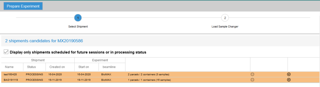
• Select the location (“basket”) in the sample changer dewar for each UniPucks in the shipment. Click the Save button after completing this step.

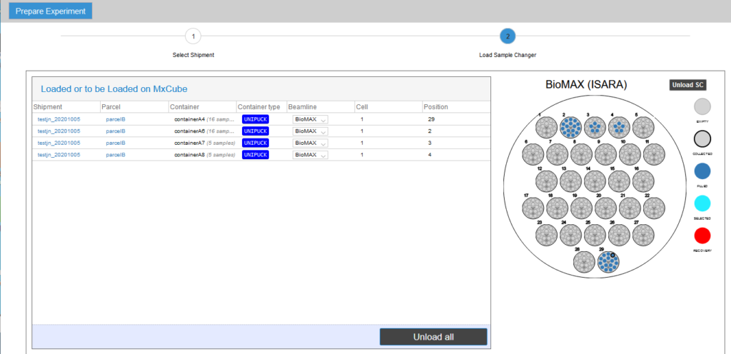
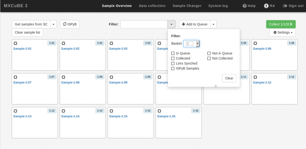
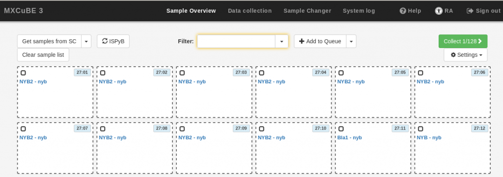
Once the pucks are assigned (manually from EXI or automatically by the IsaraLoader), go to MXCuBE3 and verify that all the sample cards are visible in the Sample Viewer menu.

It is a good idea to filter the display to list only the samples you are interested in. For example, you can filter by “basket”, which will only list the samples in the UniPuck placed in that,position of the sample dewar. You can also filter by sample name, etc.

If you need to go inside the hutch after you have started robot operation, follow this procedure:

• From MXCuBe3, use the Beamline Actions drop down menu to select the “prepare_open_hutch”. This scripted action will move the sample exchanger and other beamline motors to a safe position.
• During execution of the script, a window will pop up on MXCuBE3. Do not press the “abort” button, doing so may require a robot reset by staff.
• After the procedure is finished, the “Run” button will appear at the top of the window; then it is safe to go inside the hutch.

You will also follow the same procedure to go inside the hutch to unload your samples after the experiment. Please make sure to close the dewar lid after dismounting the samples.

Mounting single samples

Once a sample information is loaded onto MXCuBE3 you can mount it by right clicking on the sample block. This displays a sample menu that displays all the possible actions for the sample.

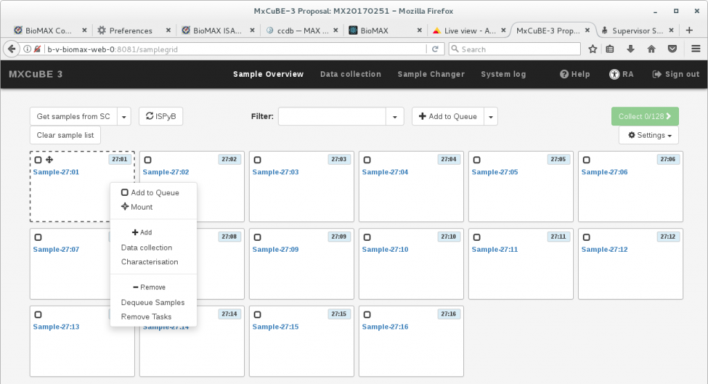
To just mount the single sample, without any setup of an automated data collection run or other sequential actions, click on Mount. If the hutch is searched, this command will also enable automatically the sample changer.

Once the sample is visible on the video screen, follow the steps in the sections below to center the sample and set up the data collection.

The rest of the selections in the menu are related to sample inclusion in a queue of automated or semiautomated tasks, as documented in the next section.

Queueing up samples and tasks

Although you can select and mount the samples one at a time, it is often more efficient to select several of them and set up a queue, which allows a number of tasks to be performed in an automatic or semiautomated sequence, while also providing the possibility to set up different tasks or data collection modes for some or all of the samples:

• Select the samples. The fastest way to do this is to click and draw a rectangle over all the samples of interest, but you can also hold down the Ctrl key and click on individual samples. The selected samples will be surrounded by a discontinuous grey frame. then, use the Add to Queue button to add all the selected samples to the queue. The samples in the queue will be highlighted in blue. To remove a sample from the queue, right click on the sample and select Dequeue sample.

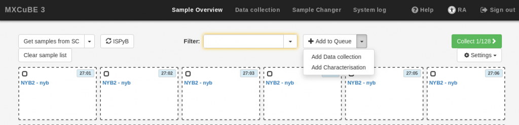
• If you wish to define characterization or data collection tasks at this point, use the Add to Queue drop-down menu, and provide the data collection parameters as described in the Data Collection section below. The same parameters will be applied to all the samples in your current selection. Note that it is not possible to execute the newly defined data collection at this stage (the Run button is inactive). If you do not want to define tasks at this stage, simply skip this step.

• Click on the Add to queue button at the bottom of the task definition box. If you added data collection parameters, a small square will be displayed on the samples in the queue for each of the task or tasks added (C for “characterization” or DC for “data collection”. You can add multiple tasks for each sample.
• If you want to remove a data collection task, click on the cross in the task button. It will also be possible to define the data collection tasks modify the parameters or add more data collections once the sample is mounted.

If you have not defined any data collection tasks, go to the Data collection Tab and click on the Mount button next to each samples to mount them and collect data one by one. Before mounting a sample, the robot will automatically dismount the previous one.

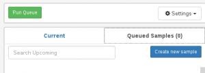
If you have defined tasks for all the samples, you can execute the queue by clicking on the Collect button in the Sample Overview tab or Run Queue in the Data collection Tab.

• A configuration pop-up window will open with some options to run the queue:

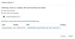
1. The Auto loop centering brings the loop into the beam and it is always run by default after mounting a sample with the sample changer . Although it is not accurate enough for data collection, it places the sample in the center of rotation and into focus and make it easier to center the crystal with the 3-click tool or with X-rays are described further below. The function also leaves the diffractometer in the “centering phase”, with a back light inserted in the beam path that makes it easier to see the crystal.
2. Select Automount next sample to dismount the current sample after all the data collections are completed and mount the following sample in the queue automatically. Only do this if you have pre-defined data collections and you have mounted your crystal so that the autoloop centering places them reliably in the beam.
3. Record crystal snapshots. You can take pictures of the crystal in up to four different orientations. The snapshots will be taken before the data collection. The first one will be shown in thesample summary in EXI.

• Click Collect when everything is OK. You will be able to stop or pause the queue execution from the Data Collection view whenever you want to change the tasks or introduce more tasks.

See the Video Tutorials Section at the end of the guide for a demo on selecting and mounting samples.

Manual sample is an option for sample mounts or containers incompatible with the sample exchanger or for collecting data at room temperature. MXCuBE3 can be used to automatically close the beamline shutter and retract the instruments surrounding the diffractometer to facilitate mounting of a new sample (this configuration is known as the Transfer phase). To set the transfer phase, use the Beamline Actions drop down menu and select “prepare new sample”. Then, go into the hutch, mount the new sample and search and lock the hutch.

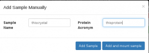
Once the sample is mounted, provide names for the sample and the protein in the respective input boxes in MXCuBE3:

• Select the Queued Samples tab and click on the button named Create new sample
• Click Add sample and mount. This will create an entry for the sample under the Current tab. If you click Add sample instead, the sample will just be added to the queued samples list, and you will have to “mount” it by clicking on the button next to the sample name. If you do not like the name you have created or you think that the sample does not look right and do not want to proceed to image collection, click Finish to remove it.
• These names will be the base for the dataset files and data storage directory names, so you may not use any spaces or strange characters; if the input box remains lined in red, the chosen name is not valid.
• Once you have mounted the sample, return to MXCuBE and change the diffractometer phase to Centring. Follow the steps described in the next section to bring the sample into focus and inspect it visually before proceeding with data collection.

• The sample exchanger mount procedure changes the phase automatically to centring mode after mounting a new sample. In the centring phase, a backlight is inserted to make it easy to see the crystal and the sample moves close to the center of the camera view, provided that the length of the pin is standard. If the crystal is far away from the beam position (marked with a blue circle), right click on the crystal or, if not visible, on any portion of the pin or the mount that you can see on the screen and select Move to beam. Use the arrows next to the Omega input box to rotate the motor by 90 degrees and adjust the sample position in the other direction. You can also access the Move to beam function by holding the Shift key and double clicking on the point you wish to center; or translate the sample using the arrows on the translation tool located to the left of the screen.

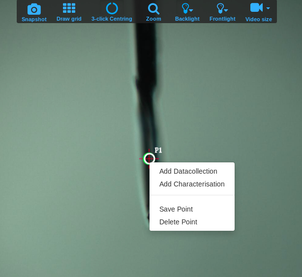
• Click on the icon named 3-click Centring to centre the sample in three clicks. Once the crystal is roughly centered at low zoom level, click on the Zoom icon to magnify the image or by holding the Z key and using the mouse scroll wheel. Adjust the centering if necessary with a new 3-click center. note: the first click will not do anything in terms of centering the crystal, it just reactivates the 3-centring function! After the centering is done, the point will be displayed in white. Make sure that you do not click on the 3-centring icon again, this will lose the coordinates for the centered position and you will have to recenter again in order to set up data collection.

• It is a good idea to rotate Omega to make sure that the crystal remains in the beam at all orientations. You can use the arrows next to the input box to rotate the motor in 90 degree steps as mentioned above; you can also change the step size by entering a different number next in the input box to the right of the motor position; or hold down the R key and use the mouse scroll wheel.
• Check that the beam size is set to the correct value. In the general case, the beam should match as closely as possible the crystal size. The diameter of the blue circle on the video corresponds to the size of the aperture, so it is easy to see which one matches best the crystal size. The default focus size at BioMAX is 50 microns. If your crystals are nearly or larger than 0.1 mm, change the focus  to 100 micron (this will also automatically select the 100 microns aperture). For crystals below 0.1 mm and above 0.015 mm use the 50 micron beam focus and an aperture of 50 or 20 microns. For very small crystals, it is best to use the fully focused beam and a 10 micron aperture. We recommend not to use the 5 micron aperture except for Synchrotron Serial Crystallography (SSX) data collection.
• Save the current position, by right clicking inside the point and selecting Save point. Saved points are displayed in green.
• To set up a data collection from the newly centered single point you can either save it or just select either Add Characterization, Add Datacollection or any of the other options available from the right-click menu. You can move to any previously saved point by clicking on it.
• If you right click outside the point you will have access to a different menu to collect 2D data (without rotating the crystal). This option can be useful to locate a good diffraction spot on an inhomogeneous crystal or determine a difficult-to-see crystal location.
• If you cannot see the sample clearly in all orientations, you can also use the X-ray centring procedure described in the next section.

See the Video Tutorials Section at the end of the guide for a demo on the three-click procedure.

The mesh scan can be used for X-ray based crystal centering, as well as fixed-target based SSX (Synchrotron Serial Crystallography) experiments. A new interface allows setting up of a semiautomated procedure for 3-D centering , which scans the crystals at two different orientations and created a 3-D centring spot.

Setting up a mesh scan

• After mounting a sample on the goniometer, center approximately the loop or mount tip with three click centering– if the sample is mounted by the sample changer, just wait for the auto loop centering to run.
• Rotate omega until you find a good orientation: for centering, you want the camera to face the direction where you cannot see the crystal (a typical example is the side of the loop for thin plates). For SSX, the chip or mount should be face side on to the camera.
• Select a beam aperture for the scan: As a rule of thumb, use an aperture half the size of your crystal. As for the beam focus, it is better to leave at 50×50 or 100×100 for larger crystals. If your crystals are smaller than 20 microns, use the fully focused beam (20 x 5 microns) together with the 5 or 10 microns aperture.
• Click the draw grid icon (next to the 3-click centering) and draw the grid by drag-and-dropping over the area you want to collect. Only works from top-left to bottom-right.
• Right click on the grid and save it.

If you right click on mesh scan, you will see an option called X-ray centering. Select this item to execute the whole procedure for 3-D centering of the crystal using a grid scan, a line scan in an orthogonal orientation and final selection of a 3-D point. If you want to do a mesh at a single orientation select mesh scan. For either method, a collection window will pop up, to set up the resolution and transmission as in other collection methods.

• Exposure time: The default of 0.011 seconds is usually fine.  However, you may have to increase it if you use a large beam size (eg. 50 microns or 100 microns) for the scan, since the diffractometer cannot translate the sample by much more than 20 microns more in 11 ms. If you overstep the physical limits of the diffractometer, the scan will fail to start. You may also need to increase the exposure if you are using a very small aperture for the mesh (eg. 10 microns) in combination with a large focus (50 or 100 microns).
• Transmission: If you use the 20 or 50 micron aperture, a transmission of about 50 -100 % is appropriate. For the 10 micron aperture, use 100 % transmission, and consider increasing the exposure time as mentioned above.
• Oscillation per image: A value of 0.1 degrees is usually fine, but you may have to decrease it for extremely large grids: If the total rotation of the sample over the entire mesh is larger than 5 degrees, the software will not allow you to use the value and you will have to choose a smaller oscillation value.
• After setting up the mesh scan, either click run now or add into the queue.
• If the scan does not run or you want to scan over a different area, do not try to delete the mesh, as this can confuse the software and require a server restart to recover. You can hide the mesh instead.

Centering the crystal

If you have chosen to run the automated X-ray centring procedure, wait for the software to run. Pay attention to error messages during the execution of the scan. If the crystal does not diffract, the automated procedure will stop after the first scan. Otherwise, a line scan will be defined and carried out automatically at a crystal orientation 90 degrees away. A new centering point will be selected based on the best diffraction.

Note: As of now, the centring procedure does not calculate the optimal beam size! You have to adjust to beam size yourself after the scan. If you used a small beam size compared to the size of the crystal, the optimal centering spot may have to be adjusted slightly in order to hit the entire volume of the crystal with a corresponding sized beam.

If you use the mesh scan option at a single orientation, the crystal will move to the optimal position after the scan if the image analysis succeeds in finding diffraction spots. However,  a centring point is not generated. You will simply see that the blue circle does not longer coincide with the initial centered spot. You can use the heat map to evaluate and readjust the position. If the heat map is too transparent, click on the draw grid button, right click on the mesh  and adjust the opacity. If the crystal diffracts only to low resolution the heat map contrast will be poor, but the calculated position is usually reliable.

• You may adjust the beam aperture, and, if necessary, the beam focus, based on the crystal profile you obtain from the heat map.
• If you can see the crystal in other orientations, use the best location in the grid (eg, the center of the blue circle, determined by the software, or an alternative position of your choice based on the heat map) as the first point in 3-click centering.
• If you cannot see the crystal for other omega values:
  1. Click on the blue circle to create a 2D point. If you want to choose a different point in the heat map as the center, right click on it and select “centring point” to create a 2D point; and then right click on the point and “go to position” to move the 2D point to the center of the beam. It may be useful to make a note of the omega angle in this orientation in case you want to restart the procedure later on.
  2. Move omega 180 degrees away to verify that  the 2D point remains centered. If this is not the case, it means that the axis of rotation is off, and you need to perform click to center procedure (click on an arbitrary position in the perpendicular orientation and the 2D point on the first and third clicks). This should not be necessary if the initial autocentering ran successfully.
  3. Rotate omega again by 90 degrees and set up a new horizontal line grid scan (you already know where the crystal is along the omega axis, so there is no need to scan in the vertical direction in the new orientation). Hide the first grid scan, as it may be difficult to right click on the new mesh if they superimpose. After the grid scan at the second orientation, the crystal will automatically move to the best point along the line. At this point the crystal is aligned to the beam at all orientations. Start the three-click centering procedure and click on the blue circle at all the three orientations.

See the Video Tutorials Section at the end of the guide for a demo on the mesh scan.

Knowing the flux (total number of photons per second on the sample) is important to be able to estimate the time that the crystal can last in the beam. MXCuBE3 will measure the flux before and after each data collection and save it under the ISPyB database experimental parameters that can be consulted from the EXI interface; it also displays the last value measured at the top of the GUI. This value will depend on the beamline transmission and the beam defining aperture in use and also depends somewhat on the beam energy. Typically, you expect to measure near 4-6×10¹² photons/s through the 50 micron aperture with the unfocused beam (50 microns) and full transmission.

For the flux measurement, the software changes the MD3 phase and translates the sample closer to the cryojet by a small amount to avoid exposing it to the X-rays. It will be returned to the original position once the measurement is finished.

If you want to measure the beam manually (for example, to check the flux after changing the energy, the beam focus or the aperture size) open the Beamline Actions and run the calculate_flux action. Note: The flux value only gets updated before each data collection or when you run the calculate_flux function. If the beam disappears afterwards, the flux value will not change automatically.

If you get a flux value of zero check for obvious causes:

• Loss of the electron beam in the R3 accelerator. Usually R3 operated at near 400 mA in frequent top-up mode. The R3 current is displayed on the top right part of the MXCuBE window, next to the safety shutter control button. If it is zero, the electron beam has been lost and there will be no X-rays reaching the sample. As of October 2023 you will also get an email to the address registered in DUO if the beam has been lost. Additionally, you can use “Get_machine_status” under Beamline Actions or check the electron beam status. After the beam has been injected (the current is close to 400 mA), open the Beamline Actions drop down menu and select “start_beamtime”. Contact staff if you get unexpected errors.
• Too high beam transmission – If you change the energy to a lower value and there are attenuation filters in the beam the transmission will decrease and can eventually become 0. Changing the transmission will let the beam through again.

If the flux readings are always zero but the diffraction images look exposed, you can continue data collection, but contact staff at the earliest convenient opportunity so that they can restart the devise that reads the flux.

The flux will change between data sets if you change the transmission, the beam size or the energy. If you have not changed any of those settings and the flux decreases sharply, You can display a live plot of the beam position in the experiment hutch with the Monitor beam icon present on the beamline workstation or remote server desktop. Clicking on the icon will open a window showing the vertical (in green) and horizontal (blue) beam positions. They both should oscillate by a around 0. If the beam position is offset from zero by more than 5-10 units the beamline could be misaligned. Try running “checkbeam” and “Align beam” from the Beamline actions menu. If neither of them succeeds in recovering the beam, contact staff.

The latest measured flux value is used for dose estimate in the data collection setup. You can also use it for a more accurate calculation, using the sample size and contents, in the raddose server.

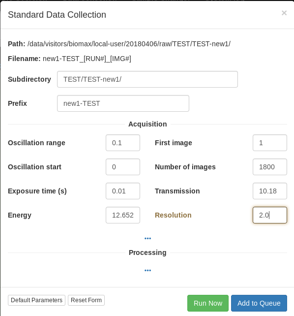
There are three different modes implemented for oscillation data collection, described below. There are also modes to to measure XRF spectra and energy scans over an absorption edge. In general, the only input required is what is displayed in the setup window when you select the desired mode.

Note that the default input values shown the first time you setup a data collection are not necessarily correct for your samples. Inspect them carefully and change them according to the recommendations below or the advice of the support person. The values you choose will be saved and selected by default for subsequent runs. If you type a parameter that differs from the current value, the input box will be lined in orange. This only means that the position of the motor will change when you start the data collection. The software will not allow you to type invalid values (for example, a value for the resolution that would result in the detector moving past its motion limit). Some optional input boxes will appear when clicking on the three dots … below the required input. Some of these options are not fully implemented yet and it is better not to use them, unless the support person indicates otherwise.

• Clicking on the Run Now button will start the data collection. Add to Queue will add it to the current queue, which can be of use when mounting samples manually to collect data from different points of the sample. Once a data collection is queued, use the Change button to modify the input parameters before the data collection is executed.
• Running data collections are displayed in blue. If you notice a problem with the data collection setup, click on the Stop button to abort the data collection fully. Stopped runs are highlighted in red. It is possible to restart stopped runs by clicking on the run and then on any of the displayed input parameters. This will reopen the setup window.
• The Pause button will stop the current action and allow you to resume the data collection, but does not have any effect once the actual data acquisition with the detector starts.
• Once the data collection is complete, it will be highlighted in green. Data collections that finish with an error are displayed in red. If the collection finishes with a warning, it will be displayed in orange.
• You can clone any run by right clicking on the run name header and selecting Duplicate from the drop down menu. The duplicated run will be then added to the end of the queue. Click on it and then on one of the input parameters to edit the data collection parameters.

Sample characterization

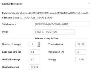
This function is used to collect up to 4 diffraction shots from a crystal at different orientations 90 degrees apart. Automated image analysis has not been implemented yet, but you can examine the images with the program Albula. A shortcut to run Albula in monitoring mode is provided in the workstation desktop.

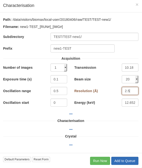
For the characterization images, it is better to collect over a wide omega oscillation to make it easier to evaluate the quality of the diffraction by eye (0.5 or 1 degree), with an exposure time of 0.05-0.1 seconds per image and transmission of 20-100%, depending on the collimator size. For the resolution, try a value somewhat better than you expect. Also beam in mind that the initial resolution from the test images, whether estimated visually or calculated by integrating the images, will often be an underestimate of the useful diffraction limit of the crystal.

Sometimes the crystals diffract to low resolution and are very mosaic as a result of a non-optimize cooling procedure. In these cases, annealing the crystal sometimes allows crystal reorganization and improves the quality. If you want to try retracting the cryojet to let the crystal warm up briefly, you can do so from the beamline actions. Note that this is a “last resort” tool and it should not be used to get rid of superficial ice from an otherwise reasonable crystal, as it will cause more damage than good in this case.

Data collection

For data collection on a single point, we recommend using exposure times of 11 ms per degree. With a defocused beam (50 microns), 0.1 degree images with 11 ms exposure per image at 20-30 % attenuation result in good quality data. We strongly recommend collecting 180 or 360 degrees, or more (in this case, please consider offsetting the kappa axis to obtain more accurate data) If the crystal is larger than the maximum available beam aperture size (currently 50 microns) it is advantageous to set up a helical data collection instead, described in the next section. For small crystals (around 10 microns) it may be better to use the focused beam with a small aperture.

The data collection calculates the estimated dose based on the current data collection parameters and a “goal” maximum dose based on the diffraction resolution and the experiment purpose (which you can select). Try never to exceed the maximum dose, unless you mean to stitch together a data set from multiple crystals. As a rule of thumb, decreasing the beam transmission is a better way to reduce the dose than reducing the number of images.

Helical scan

If the crystal is larger than the beam, the best practice to minimize radiation damage is to make the beam as large as the crystal. If you are already using the largest beam size available at the beamline, helical collection will help mitigate radiation damage by bringing a fresh volume of the crystal into the beam for each image.

To set up a helical data collection, you must define the start and end points of the data collection along the crystal. You do this by centering the crystal and saving each of the points as described above. Then, click and drag the mouse over an area including both points. That will draw a line between the points defining the data collection axis. Ideally, it is best to use two points along the omega axis, but translation along the perpendicular axis is better than collecting about a fixed point.

In cases where the crystal is not visible at one or more orientations, it is possible to do a mesh scan to locate the ends of the crystal. See, for example, this video demo.

XRF scan

The XRF scan is useful to detect the presence of heavy metals in the sample, whether they are present in the buffer or bound to the protein. In some cases, this can be useful to identify features in the density map.

When you start the scan, the fluorescence detector will move to point towards the sample. The software will acquire a series of very short exposures to determine the optimal beam transmission, which is typically rather low. Then, the crystal is exposed during the time selected in the input window (we recommend to use 0.1 seconds). The resulting spectrum will be saved to the ISPyB database. Often, the dose received by the crystal during this measurement is not higher than the equivalent of 10-20 diffraction images, but if you are concerned about minimizing the dose, you can collect it after data collection, or use a poor quality sample.

The result file will be stored together with the diffraction images in the sample directory. Besides the h5 format file, we also save a png file for easier visualization. This file is also visible in EXI.

Energy scan and SAD/MAD data collection

If a heavy atom is present in the sample and the absorption edge is within the energy range of the beamline, it is possible to do an energy scan to locate the position of the absorption edge (different, in the general case, to the theoretical value).

Tip: Before you start the energy scan, we recommend moving the energy near the absorption edge position. This will save you a little time since you will need to characterize the crystal diffraction and collect data near that energy, since the energy will move automatically back to the starting position after the scan is finished.

To start an energy scan, select the option from the right-click menu associated to a point. A periodic table will then show up. You need the select the element of interest. If you select an element with L edges, the L3 edge will be scanned. As for the XRF scan described above, the software will acquire a series of very short exposures to determine the optimal beam transmission at an energy close to the absorption edge. Then it will carry out the energy scan itself and will write out the results to the ISPyB database. Please inspect carefully the output image file in EXI, since the program used for analysis (Chooch) can fit incorrectly a very poor or non-existing signal. EXI will also list the energies corresponding to the maximum f” (‘peak’), minimum f’ (‘inflection’) and maximum f’ (‘remote’)

See the Video Tutorials Section at the end of the guide for a demo of the energy scan.

When you create a data collection following a scan, you can cut and paste the relevant energies listed in EXI; make sure that you enter the energies in MXCuBE with all the significant digits, since for some energies at or near the absorption edge, a change of 0.001-0.002 keV can have a large effect on the signal. If you create the data collection from the same sample immediately following the scan you will be also able to select one of the three energies from a drop down menu in the data collection setup window.  The energy will change automatically to the value in the input box for data collection.

To do a SAD experiment, select the ‘peak’ energy.  Typically, high multiplicity is required for successful SAD phasing. Use the dose calculation in the data collection modal to avoid exceeding reasonable doses. Remember that collecting data to the highest resolution observable is not always useful for phasing, so reduce the exposure if needed. Collecting an additional data set with a offset kappa angle can increase the accuracy of SAD data. You can do an interleaved SAD data collection at two “inverse” (separated by 180 degrees) orientations to decrease the effect of radiation damage on the anomalous signal, as described further below.

For MAD, we recommend doing a low dose data collection (for example 5-15 % transmission with a 50 micron beam) at at least two of the energies selected by the energy scan analysis, one of which should be the remote. Eg: collect 180-360 degrees at the peak or inflection energy, and then at the remote. High multiplicity is helpful, but often not so critical as for SAD phasing, since MAD phasing is intrinsically more robust. In difficult cases or P1 symmetry collecting additional data may be of helpful. We strongly recommend interleaved data collection for MAD data sets.

Interleaved data collection

Also known as “wedge” data collection, this data collection mode is used to collect pairs of reflections providing anomalous differences close in time to minimize the effects of radiation damage. The data sets are divided in angular wedges. Each wedge is collected at all the energies in an interleaved MAD data set or at different orientations in a SAD data set before proceeding to the next wedge.

To set up an interleaved data collection:

1. define a normal data collection the usual way, at the peak energy for SAD or any of the remote, peak o inflection energies for a MAD data collection.
2. Queue the data collection.
3. Click on the newly defined data collection and duplicate it. Edit the duplicated data collection and change the energy (for MAD) or the starting angle (180 degrees away) for SAD. Duplicate the run again if you wish to collect MAD data at a third energy. Queue all the data collections
4. Select all the data collections by holding the Ctrl key while you click on each of them; right-click over the ensemble and select interleaved data collection.
5. Set up the angular wedge. Note that the smaller the wedge the longer the data collection will take. Usually it is OK to use 5 to 10 wedges at each data set, but try not to exceed a dose of 1MGy per wedge over all the data sets. For example, if you are collecting two 360 degree data sets and the estimated dose is around 2.5 MGy for each data set,  you could do wedges of 75 degrees. If you wanted to collect three data sets, the maximum wedge size would be 47.5 degrees.
6. Execute the data collection.

The wedges belonging to each energy or interleaved data set will be repacked together, and the resulting data set will be renamed. The separate wedge files are stored in a separate subdirectory.

To collect crystal snapshots, click on the Snapshot icon. Make sure that you are in the centring phase, since it provides the best view of the crystal. After you have collected the snapshot, you can save the file to any location in your directories.

To have snapshots taken automatically during data collection, use the Settings pull down menu. You can take up to 4 snapshots.

Once a data collection is finished, the software will launch several automated data processing pipelines. The results can be browsed both in the ISPyB and EXI interface. At the moment, only the ISPyB interface is accessible from MXCuBe3; to access it, select the completed data collection run and click on the ISPyB link. The ISPyB application will open in another browser tab. The first time you open you need to type in your user account name and password to log in. Once logged in, go back to the tab where MXCuBE3 is running and click on the link again. ISPyB will remember your credentials and take you directly to the results page for the selected data collection.

Please also see Inspecting Processing Results using EXI.

If you want to process the data manually, see Data handling and processing at BioMAX.

MXCuBE3 supports multiple user log in from multiple locations, at the beamline or remotely. Any user belonging to the same proposal can be logged in simultaneously, although only one can issue commands and has control over the interface; this user is called “master”; by default, the master is the user who logs in first. The users who log in afterwards are “observers”. When one more than one user is logged, the number of observer users is displayed on top of the link to the Remote Access (RA) tab, and an icon to the chat tool appears to the right bottom of the interface. The RA tab lists all the users logged in and who is the current master.

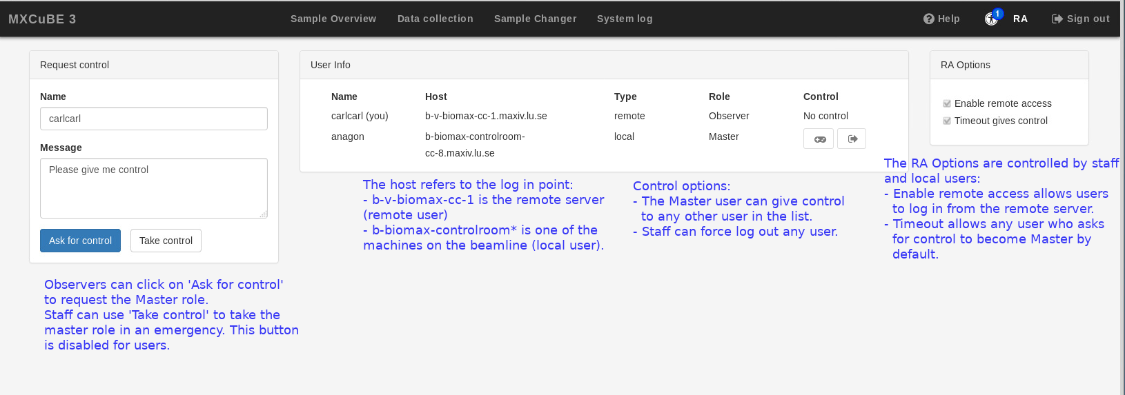
The master user should be able to mount samples, collect data and control the beamline through MXCuBE regardless of location. The observer users can navigate through all the MXCuBE tabs and see what the user in control is doing. They can also use remote tools such as the beamline video feed and the chat and request control through by clicking on the Ask for control button in the Remote Access (RA) tab. Observers cannot use the Take control button; only user support staff can use this button, if it is necessary for experiment support or troubleshooting.

If an observer asks for control, the master can give control by clicking on the window that appears on their instance of MXCuBE. There is also a general option to transfer control by default after a timeout period, enabled by default. Finally, the master user can also give control at any time to any other account logged in by clicking on the control icon in the last column of the user information list in the RA tab (but the master cannot log out any other user; that is also a support staff tool).

For general information about obtaining and preparing for remote beamtime, please read Remote experiments at BioMAX.

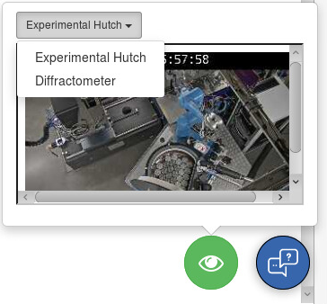
• The most common problem you are likely to encounter is a “frozen interface”, showing a fixed image on the video screen or failing to update information or messages displayed in real time (for example, you cannot see the sample rotate during three click centering or changes in the sample illumination when the diffractometer changes phase, but you can see the equipment moving if you open the beamline video feed). This lack of response is usually caused by a glitches in the connection to the video or other servers. It usually can be solved easily by refreshing the MXCuBE3 application web page. If the glitches happen very frequently, try closing the beamline video (if you have it open all the time), or reduce the number of observers logged in to MXCuBE at the same time.
• Sometimes, the interface fails to respond totally even after refreshing the browser page. In this case, find and run Restart_MXCuBE from the list of beamline actions. In some instances, you may get kicked out from MXCuBE when the server crashes; if this happens, you can restart the server from the command line: Open a terminal in the remote server and type “restart_mxcube”. After some seconds, you should be able to reopen MXCuBE and get to the login page. Note: After restarting the server you will have to rebuild the sample queue. You will not be able to see which samples you have already collected data from either. However, the sample collection information is preserved in the ISPyB database, and you can view it from the EXI Data explorer tab.
• Occassionally, MXCuBE loses the connection to ISPyB. When this happens, the data file names do no longer match the saple names in the ISPyB sample list, and the Sample view is empty. To resynchronize to ISPyB, sign off from MXCuBE and then log in again.
• If the sample changer finishes the mounting operation but there is no sample or a sample base on the goniometer, please use the beamline video to verify that there is indeed no sample mounted. If there is no sample on the goniometer: To be able to continue mounting samples, go to the Beamline actions and click the button empty_sample_mounted. It is safe to try remounting the sample in case the robot gripper just failed the first time. Other causes of an “empty mount” can be from a mistake filling up the sample information to the sample getting stuck in the puck base at loading.
• If you can see there is a sample mounted on the goniometer but at a weird angle, you must call support staff or, if you are collecting data on site, remove the sample yourself (see next point). This happens if the sample length is much longer than 22 mm and trying to use the robot to dismount the sample will cause a collision.
• If you want to log in out of MXCuBE but the Sign out button appears to be inactive, try increasing the size of the browser window. This can be a problem when running MXCuBE3 on a small screen.
• Currently MXCuBE will give an error at the beginning of the data collection if the calculated flux is 0, or if the beam has not stabilized after an energy change, but it will not stop the task. If the diffraction images look blank (no scatter from the air creating a beamstop shadow, no counts on the detector), there is likely no beam reaching the sample. The most common reason is a beam dump. Please see the section Monitoring the beam and measuring the flux to help diagnose the problem.
• If you are using the fully focused beam and observe that the flux values decrease steadily during the experiment for the same beam transmission and aperture values, try to align the beam in the beamline tool menu. This should not be necessary for larger beam sizes.
• If the data collection fails with a “Failed to arm detector” error, please check that you are not trying to collect images with the same name as a previous data collection. This can happen sometimes if you collect data from the same sample after restarting the MXCuBE server. If this is not the case and the data collection fails with this or another error, contact staff.
• If the data collection appears to finish normally but you cannot open the images or see the data in EXI, call staff.

• Mounting samples with the Sample Changer.
• Three-click center procedure.
• Gris (mesh) scan.
• Energy scan.
• Setting up a helical scan with grid scans.